

Author’s note:
The Reductive-Investment Analysis is the latest method of calculation of the investments’ effectiveness. It is a unique decision for the investment analysis of the exchange market. It guarantees a simplified understanding of the market prospects, gaining of profit and the continued success of the investor. It gives you opportunity to make a management decision on the feasibility of investment or the timely withdrawal from the market. It has an exceptional mechanism to model the dynamics of future prices. The present publication is recommended for trade floor analysts and financial experts.
INTRODUCTION
A significant part of investments in financial tools of the stock market does not provide the expected and planned result for reasons beyond the control of investor. An absurd or poor-quality investment analysis causes most of the cases resulting in losses. Against the backdrop of globalization and a certain “mutation” of the financial market, the need for new and advanced methods for the theoretical description of the mass expectations of financial market participants has grown, with possible further modelling of quotes on this basis. This paper, titled “A Reductive-Investment Analysis”, describes the results of long-term, empirical studies of the financial and stock market. It represents a new, alternative approach to assessing, analyzing and modelling in financial markets using logical techniques and such statistical software tools as a regression channel, calculated based on the least squares method.
A Reductive-Investment Analysis is a system of logical and practical approaches, methods of analyzing financial tools of the stock market (securities, currencies, derivative contracts, etc.), for the investor, substantiating and evaluating the feasibility of making investments, and optimizing investment trading operations, to make an effective decision. It is a dynamic process occurring in two planes — time and price. In the time plane, the work is carried out to monitor market expectations. They provide a steady understanding of the process of developing investment objectives. In the price plane, analysis and development of descriptive solutions in different substantive aspects are mainly carried out. These aspects include the econometric component, correctly stated objectives and tasks of investment, analysis of investment risk, and the general sensitivity to changes in certain significant factors.
The principle of the Reductive-Investment Analysis as a whole is a method to narrow the complexity one down to the simplicity, by means of logical-methodological procedures of presenting a complex process as a sequence of simple techniques. This method makes it available for analysis.
The process of Reductive-Investment Analysis comes laden with descriptive methods of converting data associated with a particular stock exchange tool in order to simplify it and present it by means of some more accurate language, as well as to model the investment objectives.
The subject matter of this analysis as a practical method is that for the solution of a complex task, the researcher narrows its structure down to a simpler version available for analysis or solution. For example, the solution of a matter in mathematics can be narrowed down to another matter, if the solution of the first one can be the solution of the second one. In logic and in the methodology of science, the reduction is usually refers to the explanation of the theory or a variety of experimental laws established in one research area, using the theory formulated for another one.
Methods and techniques of Reductive-Investment Analysis are the means for an objective research of the processes in the investment area, as well as the formulation of conclusions and recommendations based on them. The procedure and the applied methods of this analysis are aimed to propose alternative options for modelling possible processes, identifying the scale of proposed events and their actual comparison according to various efficiency criteria.
The objects of the Reductive-Investment Analysis are financial and stock tools, which are traded within online international stock exchanges.
The subjects of this analysis are users of analytical information directly or indirectly interested in the results and achievements of investment activities, owners, management, personnel of financial organizations, suppliers, buyers, creditors, the state represented by statistical and other bodies analysing information in terms of their interests to make investment decisions.
Section 1. The main characteristics, typology and principles of the Reductive-Investment Analysis
The Reductive-Investment Analysis, as a descriptive method, combines a set of theoretical techniques and models based on econometric theory, using mathematical and statistical tools (linear regression channel), providing quantitative expressions with visual perception with the further possibility of visual modelling of goals and prospects for further development of the ongoing process.
In economic researches the problems of identifying the factors that determine the dynamics of the economic process are often solved. Also, in order to reliably reflect the processes existing in the economy objectively, it is necessary to identify significant relationships and give them a quantitative assessment. This approach requires the disclosure of causal dependencies. The causal dependence means such a relationship between processes, when a change in one of them is a consequence of a change in another. The solutions of such matters most often use methods of correlation and regression analysis.
Economic data is usually presented in tabular form. The numerical data contained in the tables usually have explicit (known) or implicit (hidden) connections between them. The indicators that are obtained by direct counting methods, i.e., are calculated according to previously known formulas, are clearly connected. For example, percentages of plan fulfilment, levels, specific gravity, deviations in the sum, deviations in percentages, growth rates, accession rates, indices, etc. Connections of the second type (implicit) are not known in advance. However, it is necessary to be able to explain and predict complex phenomena to control them. For this reason, with the help of observations, specialists seek to reveal hidden dependencies and express them in the form of formulas, mathematically simulate phenomena or processes. One of such opportunities is provided by the correlation and regression analysis. Mathematical models are built and used for three generalized purposes: explanation, prediction and control. The presentation of economic and other data in spreadsheets or through the tools of trading platforms has become ordinary and widespread these days. Equipping electronic trading platforms with the means of correlation and regression analysis gives specialists in the financial field opportunity to transform well-founded probability-theoretic methods into everyday effective analytical tools. Using the tools of correlation and regression analysis, analysts measure the linear statistical dependence of the indicators by means of the correlation coefficient. This reveals the connection, different in strength and direction. Regression analysis is one of the main methods to identify implicit and covert connections between observational data in modern mathematical statistics.
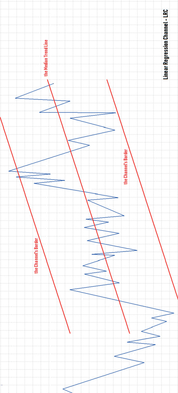
Mastering the technique of using tools based on regression analysis, you can apply it as needed, gaining knowledge about hidden connections, improving analytical decision-making support and increasing their validity. Thus, the methodology of the Reductive-Investment Analysis is a research method closely related to the tools of correlation and regression analysis, which is based on the use of the Linear Regression Channel tool (Fig. 1) available in modern electronic trading platforms. The Linear Regression Channel is built based on the Linear Regression Trendline, an ordinary trend line built between two points on the price chart using the least squares method. This method calculates the Y=a+b*X trend line, minimizing the sum of squares of vertical deviations between the closing price value and the trend line value during a given time interval. The trading platform software calculates the values (a, b) and builds a Linear Regression line for any time interval. As a result, this line turns out to be the exact median line of the changing price.
The Linear Regression Channel, developed by Gilbert Raff in 1991, consists of two parallel lines equidistant up and down from the linear regression trend line. As a result, the Linear Regression Channel consists of three parts: the median line is the trend line; the upper and lower lines are the borders of the Linear Regression Channel. The distance between the borders of the channel and the median trend line is equal to the maximum closing price deviation from the median line of the Channel (Fig. 1).
A Reductive-Investment Analysis is a multidimensional method applied for the visualization of the interrelation between the values of quantitative variables. The basic idea of the concerned analysis lies in the fact that available dependencies among large number of initial observable variables give us opportunity to analyze the development of phenomena in time. The methods of the Reductive-Investment Analysis make possible not only to explore the data, but also to choose a method for their further in-depth analysis for examination of the statistical hypotheses and modelling of the further dynamics. In the current analysis, the price information about the examined phenomenon is shown in aggregated form by means of graphic tools. The main objective of the Reductive-Investment Analysis is the modelling of both the future development of the further financial market dynamics by means of descriptive tools, and the corresponding actions of the market participants meant to simplify the analysis procedures.
Section 2. Methodology of a Reductive-Investment Analysis
Module 1
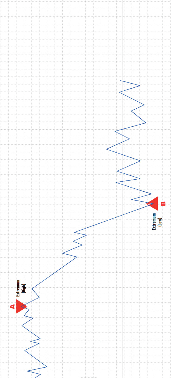
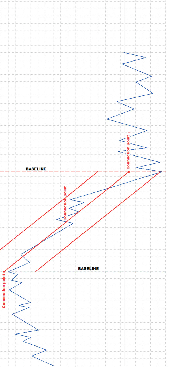
The algorithm of the Reductive-Investment Analysis consists of a sequence of clearly aligned Linear Regression Channels, their modelling relative to the current trend. The modelling process starts with the identification of price extremes. For a bearish trend the counting is started from the high price to the low price, from A to B (Fig. 2), while the bullish trend, on the contrary — from the minimum to maximum. Price extremes are the starting points to fix vertical baselines. Vertical baselines are the stationary levels to which the connection points of the Linear Regression Channel are attached (Fig. 3). First of all, the stationary Linear Regression Channel is fixed to the baselines, the minimum of the median line of which (D point, Fig. 4) possesses the function of the point relative to which the breakout line is drawn. Further constructions of the regression channels happen in the process of price consolidation of the asset in question. According to the market laws, after a significant price movement from extreme to extreme, temporary consolidation is sure to occur. This is a state where the prices of stock assets do not have a clearly defined trend and move in a narrow price range due to the fact that the supply and demand for a particular stock asset in the market are approximately equal. In the process of such price consolidation, the next Linear Regression Channel is used, sliding with the price and is intended for visual monitoring and identification of possible regression deviations (Fig. 4). With the usual price dynamics, the median line of the Linear Regression Channel moves evenly with the price, simultaneously updating current extremes with it. But it sometimes happens that during consolidation periods, after significant unidirectional price movements from extremum to extremum, the lateral correction, with the oscillation dynamics different from most cases, separates the price direction and the median line of the Linear Regression Channel (Fig. 4). In such cases, a financial tool is taken for development, designed to identify a suitable investment environment by visual modelling and tracking the general view of price movements. Further, when during prolonged consolidation the median connection point of the sliding Linear Regression Channel reaches the right baseline, it is fixed in this position for further analysis of the current situation. If, with such a fixation, the pole of the median regression line “L” of the sliding LRC (Fig. 4), deviating from the price directivity, breaks through the Breakout Line and the Extremum Line, then a fact occurs signalling a certain deviation from the ordinary norm. Such a deviation is a consequence of the fact that unidirectional trading in the financial tool under research has reached a certain standard where market saturation occurred, or some uncertainty appeared among market participants, which may turn prices in the opposite direction. Due to the fact, that the Breakout Line and the Extremum Line are broken through by the “L” pole of the median line of the sliding LRC (Fig. 4), the “L” level becomes a historical reminder with a further corresponding conjuncture of the monitored object necessary for subjection. After identifying a non-standard situation and fixing a sliding LRC with a clear price divergence from the regression model, further monitoring of the current prices relative to the next sliding-indication LRC is continued (Fig. 5). The need for the next sliding LRC is a clear demonstration of the current situation on the road to achieving an investment-friendly event. This event is favourable for investments when the prices of the Orienting line (Fig. 6, 7) correspond to the range of 75%-85% of the backward level relative to the trend under research, with a corresponding regression model (Fig. 8). This Orienting line is drawn relative to the stationary LRC, the “W” point of the Orienting point, which is determined by the crossing of the Channel Border by the stationary LRC and the Baseline (Fig. 6, 7). The importance of this backward distance lies in the fact that it is at such amplitude that the properties of the regression models are revealed that clearly indicate any changes in the general trend of the observed financial tool. This is necessary to minimize the risks, as well as for a timely and adequate response to force majeure. The following regression construction carries with it the purpose of a visual indication of the above circumstances and changes (Fig.9). For this, the calculated Linear Regression Channel is fixed, the connection points of it are attached to the vertical baselines from right to left — first the “R” point, then the median connection point “N” (Fig. 9). This model of LRC is necessary to draw the Reference Line (Fig. 9), which is determined relative to the connection point “R” of the calculated Linear Regression Channel and carries with it the role of an indication level. With the non-standard angular directivity of the calculated LRC, in the direction opposite to the trend direction, the Reference line is fixed relative to the “T” point (Fig. 10). The Reference line clearly shows the area of location of the “K” pole of the trend line of the indication LRC (Fig. 5), when the prices of the Orienting line and 75% -85%, favourable for investments, reach the range level. If the “K” pole is located in the same area as the “L” market checklist (Fig. 4) and with the same vectorial orientation, then this is one of the confirmations of the favourableness of the event for investment actions (Fig. 5). Such a state visually reveals a discrepancy in the current trend, relative to regression models in comparison with previous models at the same prices. This discrepancy indicates changes in the interests of the market participants, according to the traded financial tool, thereby signalling the maturing of a favourable environment for investment. Also, the connection point “S” of the indication LRC should be located in the area opposite to the location of the “K” pole and the market reminder “L”, forming the correct angular direction (Fig. 5). The mobility of the indication LRC, it’s sliding, parallel to current prices, allows you to monitor visually and continuously and control the current trend, visually see any changes, deviations in the angular direction of the trend, manage risks and timely detect structural inconsistencies in the overall picture of price dynamics risky for investment actions. The above-mentioned defined locations of the “S” and “K” points relative to the Reference line identify current changes. So, finding the “S” point and the “K” pole of the indication LRC in the same area relative to the Reference Line is a signal for change of the investment-friendly model and an indicator of the situation not recommended for any actions (Fig. 11). Also, for correct identification of the required model, the indication LRC is used, the beginning of construction of which is started from the baseline drawn relative to the “D” point (Fig. 12). The present indication LRC will clearly show the regression component of the consolidation process, or the average prices from the beginning of the extremum. In the consolidation process, when the mid-point “U” of the median line of the indication LRC is reached the breakout line, the “G” pole of the indication LRC should not break the Resistance line drawn from the “E” point of the median line of the sliding LRC (Fig. 12). This construction will be another confirmation of the correctness of the investment-friendly model, indicating a hidden focus in the price trend for the financial and stock tool under research. Otherwise, in the process of prolonged consolidation, when the “G” pole breaks the Resistance line, this model loses its attractiveness. During the maturation of the investment-friendly prerequisite and the formation of a structurally correct regression model for the financial and stock tool being monitored, investment and trading activities are carried out in the direction of the “L” price reminder of the market (Fig. 4, 15). This happens with the constant tracking of the indication LRC, with the aim of timely identifying the change in the current trend (Fig. 13, 14).
Module 2
Because of the supply and demand dynamics, the price of a particular asset traded on the financial markets, or the stock, fluctuates along a certain trajectory, driven by news and the mood of the crowd. High liquidity of exchange assets allows using them as the means of investment, and high volatility, compared to other over-the-counter goods, attracts to the market not only long-term investors, but also short-term speculators, whose interest is only in investing funds, although with high risks, but for profit in the near future. Thus, investors and speculators significantly deviate the price of an asset from “fair”, creating demand and supply, depending not on an objective assessment of fundamental indicators, but on expectations of a change in price. These expectations can be based on the expected changes in indicators, such as rumors, and may just correspond to the current or estimated price dynamics. The law of economics says that under equal conditions, the lower the price of a product, the greater the demand and the lower the supply. But the speculative demand for an exchange asset is subject to completely different laws, its dependence on price has completely different properties. The low price of any asset can’t provoke mass demand if the majority of traders are set to further decline. The expectations of traders about the further development of events have great importance. If the majority believes that the price will rise and start to purchase it, no objective assessment of the “fair price” will keep it from rising. And if the movement is strong enough, psychological mechanisms start to operate, which further increase the movement. In the case of the price break, traders tend to get rid of the asset trending downward rapidly and increase the already strong supply, so the trending downward will be until the majority decides that they are downward far enough and a further decline is unlikely. Similarly, with strong growth, more and more traders become interested in growth and enter the game on the growing market side, increasing already significant demand. And often panic sales are quickly replaced by equally panic purchases. It would seem that one can expect price fluctuations near the “fair” even in the long-term period; however, in fact, the price can be both higher than fair as long as it can, and even lower. Such endogenous demand and supply, formed within society among market participants, is a favourable environment for modelling investment objectives and further processes, subject to minimal exogenous influences on the market, not interference by the governments and forces from outside.
The following model of the Reductive-Investment Analysis structures the values of the current processes, to simulate the prospects for the proposed events, during the formation of post-backward consolidation. As in the case of the first model, the modelling process starts with the identification of price extremes. For the bear trend the observation is made from the high price to the low price, from A to B (Fig. 2), while for the bull trend, on the contrary, it is made from minimum to maximum. Further, the Linear Regression Channels are established sequentially in relation to the vertical Baselines. The connection points of the LRC-1 middle line are fixed from right to left, first the “D” point, then the “C” mid-point (Fig. 16). The connection points of the LRC-2, “F” point and “G” mid-point are fixed to the Baselines from left to right (Fig. 17). This construction shows the development of the current trend in time, the delaying of the backward procedure, the entry of the stock exchange quotation into the consolidation stage after the rise or fall. Fixation of LRC-1 and LRC-2 is the basic structure in the process of modelling by regression channels, for which further actions are performed. To the Baseline drawn through “G” and “D” connection points from LRC-1 and LRC-2, LRC-3 is fixed by means of connection point “H”, extending to the Baseline drawn relative to the connection point “E” of LRC-2 and fixing to it with the mid-point connection point “R” of LRC-3 (Fig. 18). This action is needed to identify the maximum regression level relative to which the Resistance line is established. In this case, this line is drawn through the connection point “P” of LRC-3 (Fig. 19). Further, to the Baseline drawn relative to the connection point “F” and the mid-point “C” from LRC-2 and LRC-1 respectively, the LRC-4 is fixed by means of the connection point “M” and extends from right to left to the next Baseline through connection point “L” of LRC-1, fixing to it by means of the mid-point “U” of LRC-4 (Fig. 20). After fixing the LRC-4, the connection point “M” of this Linear Regression Channel becomes the reference point for the next Resistance line (Fig. 21). In the use of this model, the Resistance lines act as indicator levels, showing the favourable trends for investment actions, and also when they break through with regression median lines signal a change in trends. The following Linear Regression Channel LRC-5 is fixed to the Baseline passing through the mid-point “R” of LRC-3 and connection point “E” of LRC-2 through the connection point “K” of LRC-4, fixing to it with the mid-point “T” of LRC-5 (Fig. 22). This action is needed to identify the level for one of the Reference lines. So, this line is drawn through the connection point “S” of LRC-5, relative to which the calculated measurements will be carried out (Fig. 23). Further, to identify the next levels required for the next Reference Line, the following Linear Regression Channel LRC-6 is drawn (Fig. 24). Its fixation is carried out respectively from right to left of the Baseline passing through the connection point “P” of LRC-3, fixing itself with the connection point “Z” of LRC-6, extending to the Baseline through the connection points “F” of LRC-2, “M” of LRC-4 and mid-point “C” of LRC-3, connecting with it in the mid-point “Y” of LRC-6 (Fig. 24). After that, the Reference line is drawn relative to the fixed connection point “Z” of LRC-6 (Fig. 25). Also, the following Reference lines are carried out relative to the mid-points “U” of LRC-4 and “R” of LRC-3 (Fig. 26) and the Resistance line relative to the fixed connection point “L” of LRC-1 (Fig. 27).
As in the module 1, the indication LRC is used to identify the necessary investment-friendly model. In this case, it is LRC-7, the construction of which starts from the baseline drawn relative to the “K” point of LRC-4 from left to right (Fig. 28). This indication LRC will clearly demonstrate the regression component of the current consolidation process, the discrepancies between the highs and the average prices on the regression channels.
In the consolidation process, when the Reference lines reach the mid-point “J” of the indication LRC-7, drawn from “U”, “Z”, “S” and “R”, the “B” pole of the indication LRC-7 should not break the resistance lines drawn from the “L”, “M”, “P” points of median LRC-1, LRC-4, LRC-3 (Fig. 29). This construction will be another confirmation of the correctness of the investment-friendly model, indicating a hidden focus in the price trend for the financial and stock tool under research. Otherwise, in the process of prolonged consolidation, when the “B” pole breaks through the Resistance lines, this model loses its investment and trade attractiveness. In addition to the indication LRC-7, the LRC-8 is drawn, which performs the same indicator function when modelling current processes, to display connections between the regression price data with different time intervals (Fig. 30). This LRC-8 originates from the Baseline drawn through the connection point “S” of the LRC-5 and the median “R” of the LRC-3. Thus, in the process of reaching the Reference lines by the median point “J” of the indication LRC-7, the “N” pole of the indication LRC-8 should not break through the Resistance lines. In this case, the poles of the two indication LRC should intersect, signalling favourable conditions for trading actions with the opposite direction (Fig. 30). The time limit of the trading cycle is achieved when the mid-point “J” of the indication LRC-7 horizontally crosses the Baseline from left to right (Fig. 31). It shows uncertainty in the actions of market participants, the lack of focus in price dynamics, the decrease in demand for an asset in anticipation of important events. In this case, trading actions are recommended to be suspended.
Module 3
The model of the third module of the Reductive-Investment Analysis is based on the structure of the previous model of the second module, with a slight difference in the use of one of the Regression channels, for modelling of the prospects for the alleged events in the formation of post-backward consolidation. As in the case with previous models, the modelling process starts with the identification of price extremes. In this case, in a bullish trend the counting is started from the low price to the high price, from A to B (Fig. 32). Further, relative to vertical Baselines, drawn from price extremes, the Linear Regression Channels are sequentially established. From right to left, the connection points of the median line of LRC-1 are fixed, first the “D” point, then the mid-point “C” (Fig. 33). From the left to the right, the connection point “F” and the mid-point “G” are fixed to the Baselines, from LRC-2 (Fig. 34). This construction demonstrates the development of the current trend in time, the inhibition of the backward process, the entry of the exchange rate into the consolidation phase after a rise or fall. And in this model, the fixation of LRC-1, LRC-2, is the basic structure in the process of modelling by regression channels, with respect to which further actions are performed. To the Baseline drawn through connection points “G” and “D” from LRC-1 and LRC-2, LRC-3 is fixed by means of connection point “H”, extending to the Baseline drawn relative to connection point “E” of LRC-2 and fixing to it with the median connecting point “R” of LRC-3 (Fig. 35). This action is needed to identify the minimum regression level relative to which the Resistance Line is established. In this case, this line passes through the connection point “P” of LRC-3 (Fig. 36). Further, the LRC-4 is fixed by means of the connection point “M” to the Baseline drawn relative to the connection point “F” and the mid-point “C” from LRC-2 and LRC-1 respectively, and extends from right to left to the next Baseline through connection point “L” of LRC-1, fixing to the mid-point “U” of LRC-4 (Fig. 37). After fixing the LRC-4, the connection point “M” of this Linear Regression Channel becomes the reference point for the next Resistance line (Fig. 38). Just as in the previous model, the Resistance lines act as indicator levels, showing the favourable trends for investment actions, as well as when they are broken through with regression median lines they are signalling a change in trends. The following Linear Regression Channel LRC-5, through the connection point “S”, is fixed to the Baseline passing through the mid-point “R” of LRC-3 and connection point “E” of LRC-2 and extends from right to left to the Baseline through the connection point “K” of LRC-4, fixing to it with the mid-point “T” of LRC-5 (Fig. 39). This action is needed to identify the level for one of the Reference lines. So, this line, relative to which the calculated measurements will be made, is drawn through the connection point “S” of LRC-5 (Fig. 40). Further, to identify the next level required for the next Resistance line, the following Linear Regression Channel LRC-6 is drawn (Fig. 41). Its fixation occurs respectively from right to left of the Baseline passing through the connection point “P” of LRC-3, fixing itself with the connection point “Z” of LRC-6, extending to the Baseline through the connection points “F” of LRC-2, “M” of LRC-4 and mid-point “C” of LRC-1, connecting with it in the mid-point “Y” of LRC-6 (Fig. 41). After that the Resistance line is drawn relative to the fixed connection point “Z” of LRC-6 (Fig. 42). Also, the following Reference lines are drawn relative to the mid-points “U” of LRC-4 and “R” of LRC-3 (Fig. 43), as well as the Resistance line, relative to the fixed connection point “L” of LRC-1 (Fig. 44).
Further, to identify the necessary investment-friendly model, the indication LRC is used. As in the model of the second module, this is an indication LRC-7, the beginning of construction of which is started from the Baseline drawn relative to the “K” point of the LRC-4 from left to right (Fig. 45). This indication LRC will also clearly demonstrate the regression component of the current consolidation process, the relationship and discrepancies between the minima and average prices on the regression channels.
In the process of consolidation, when the mid-point “J” of the indication LRC-7 reaches the Reference lines drawn from “U”, “S” and “R”, the “B” pole of the indication LRC-7 should not break through the Resistance lines drawn from the points “L”, “M”, “P”, “Z” of median LRC-1, LRC-4, LRC-3, LRC-6 (Fig. 46). With such a construction, the correctness of the investment-friendly model will be confirmed, showing that the change of direction is maturing in the price trend for the financial and exchange tool under study. Otherwise, in the process of prolonged consolidation, when the “B” pole breaks through the Resistance lines, this model loses its investment and trading value. In addition to the indication LRC-7, the LRC-8 is drawn, which performs the same indication function when modelling current processes, to display the relationships between the regression price data with different time ranges (Fig. 47). The present LRC-8 originates from the Baseline through the connection point “S” of LRC-5 and the median “R” of LRC-3. So, in the process of reaching the Reference lines by the point “J” of the indication LRC-7, the pole “N” of the indication LRC-8 also should not break through the Resistance lines. In this case, the poles of the two indication LRC should intersect, signalling favourable conditions for trading actions with the opposite direction (Fig. 47). The time limit of the trading cycle is achieved when the Baseline is horizontally crossed by the mid-point “J” of the indication LRC-7, from left to right (Fig. 48). This is one of the signs showing the vagueness in the market makers’ actions, the lack of focus in price dynamics, the decline in demand for an asset in anticipation of important events. In such a case, trading activities are also recommended to be suspended.
Module 4
The Regression model of the fourth module of the Reductive-Investment Analysis shows the interrelation of the values of each of the segment of the basic construction of the regression channels, when modelling the prospects for the intended events, for certain trading actions. As in the previous models, the modelling process starts with the identification of price extremes. In this model, the counting is conducted from the high price to the low price, from A to B (Fig. 49), with respect to which the basic Baselines are drawn. Further, the Linear Regression Channels are sequentially established with respect to these Baselines. From right to left, the connection points of the median line LRC-1 are fixed, first the “D” point, then the median point “C” (Fig. 50). From left to right, connection points from LRC-2, “F” and median “G” are fixed to the Baselines (Fig. 51). This construction shows the development of the current trend in time, the inhibition of the backward process, the entry of the exchange rate into the consolidation stage after a rise or fall. To the Baseline drawn through connection points “G” and “D” from LRC-1 and LRC-2, LRC-3 is fixed by means of connection point “H”, extending to the Baseline drawn relative to connection point “E” of LRC-2 and fixing to it with the median connecting point “R” of LRC-3 (Fig. 52). The need for this action is to identify the regression level, relative to which the Resistance Line is established, which is drawn through the connection point “P” of LRC-3 (Fig. 53). Further, to the Baseline drawn relative to the connection point “F” and the mid-point “C” respectively from LRC-2 and LRC-1, the LRC-4 is fixed by means of the connection point “M” and extends from right to left to the next Baseline through connection point “L” of LRC-1, fixing to it with the mid-point “U” of LRC-4 (Fig. 54). After fixing the LRC-4, the connection point “M” of this Linear Regression Channel turns into the reference point for the next Resistance line (Fig. 55). When modelling the price dynamics of an exchange asset, the Resistance lines act as indication levels, consolidation below which shows a favourable trend for trading actions, as well as their breaking through by regression medians, signalling a change in trends.
The following Linear Regression Channel LRC-5, through the connection point “S” is fixed to the Baseline passing through the mid-point “P” of LRC-3 and extended to the Baseline through the connection point “U” of LRC-4, fixing to it with a “T” point of LRC-5 (Fig. 56). This action is needed to identify the levels for carrying out the Reference lines. So, these lines are drawn through connection points “S” and “T” of LRC-5, relative to them the calculated measurements will be made (Fig. 57). Further, to identify the next levels required for the subsequent Reference lines, the following Linear Regression Channel LRC-6 is drawn (Fig. 58). It is fixed by the connection point “Z” to the Baseline passing through the mid-point “R” of the LRC-3, reaching up to the Baseline through the connection point “K” of the LRC-4, connecting with it in the “Y” point of LRC-6 (Fig. 58). After that the Reference lines are drawn relative to the fixed connection points “Z” and “Y” of LRC-6 (Fig. 59, 60). Subsequent Reference lines are drawn relative to both connection points of LRC-2 (“F”, “E”), mid-points of “R” of LRC-3 (Fig. 61), “C” of LRC-1 (Fig. 62), “U” of LRC-4 (Fig. 63), as well as a Resistance line is drawn relative to the fixed connection point “L” of LRC-1 (Fig. 63).
To identify the correct investment-friendly model, the indication LRC-7 is used, the construction of which starts from the Baseline drawn relative to the “K” point of the LRC-4 from left to right (Fig. 64). Indication LRC in the process of price advancement will visually signal a divergence between the maximum and average prices on the regression channels of the current consolidation process.
When the exchange rate is stabilized and the mid-point “J” of the indication LRC-7 reached the Reference lines drawn from “T”, “S”, “Z”, “Y”, “R”, “E”, “F”, “C”, “U”, the “B” pole of the indication LRC-7 should not break through the Resistance lines drawn from the points “L”, “M”, “P” of the median LRC-1, LRC-4, LRC-3 (Fig. 65). Such a construction shows the divergence between the values of average and maximum prices from the regression coefficients, when the price levels of the investment under consideration reach new average upward values, but the maximum indicators can’t reach the peaks of the previous levels. This will be a confirmation of the profitability of the current model for certain trading actions, showing the maturity in the price trend of the inevitable reversal of the financial and exchange tools being under study. Otherwise, in the process of protracted consolidation, when the “B” pole breaks through the Resistance lines, this model loses its investment and trading attractiveness. In relation to the indication LRC-7, the LRC-8, with a short time range, is performing the same indication function when modelling current processes, to display the relationships between the regression price data with different time ranges (Fig. 66). The present LRC-8 originates from the Baseline through the connection point “E” of the LRC-2, “Z” of the LRC-6 and the median “R” of the LRC-3. Thus, in the process of reaching the Reference lines with the mid-point “J” of the indication LRC-7, the “N” pole of the indication LRC-8 should not break through the Resistance lines. In this case, the poles of the two indication LRC “N” and “B” should intersect, signalling favourable conditions for trading actions with the opposite direction (Fig. 66). The time limit for the trading cycle is achieved when the Baseline of the midpoint “J” of the indication LRC-7 is horizontally crossed from left to right (Fig. 67), which, in turn, may be due to uncertainty in the actions of market participants, the lack of significant drivers or decrease in demand for one or another asset before the release of important information. In this case, it is recommended not to take trading actions.
Module 5
The model of the fifth module of the Reductive-Investment Analysis gives opportunity to smooth price regression drawbacks in channel modelling, to identify base levels by rotating the LRC, and also allows the use of additional channels for detailing constructions. The modelling process starts with the identification of price extremes and fixing baselines. In this case of a bullish trend the counting is conducted from the low price to the high price, from A to B (Fig. 68). Regarding the vertical baselines, the Linear Regression Channels are sequentially established. From right to left, the connection points of the median line LRC-1 are fixed, first the “D” point, then the mid-point “C” (Fig. 69). From left to right, to the Baselines, the connection points “F” and “G” are fixed, from LRC-2 (Fig. 70). Fixation of LRC-1 and LRC-2 is the basic structure at the beginning of the construction of the regression channels, for which further actions are carried out. To the Baseline drawn through connection points “G” and “D” from LRC-1 and LRC-2, LRC-3 is fixed by means of connection point “H”, extending to the Baseline drawn relative to connection point “E” of LRC-2 and fixing to it with the median connection point “R” of LRC-3 (Fig. 71). This action is needed to identify the minimum regression level relative to which the Resistance Line is established. This line is drawn through the connection point “P” of LRC-3 (Fig. 72). Then, to the Baseline drawn relative to the connection point “F” and the mid-point “C” respectively from LRC-2 and LRC-1, the LRC-4 is fixed by means of the connection point “M” and extends from right to left to the next Baseline through connection point “L” of LRC-1, fixing to it with the mid-point “U” of LRC-4 (Fig. 73). After fixing the LRC-4, the connection point “M” of this Linear Regression Channel becomes the reference point for the next Resistance line (Fig. 74). As in the previous models, the Resistance lines act as indication levels, the limits of which show a favourable trend for investment actions and their breaking through by regression median lines signal a change in trends. The following Linear Regression Channel LRC-5, through the connection point “S”, is fixed to the Baseline passing through the mid-point “R” of LRC-3 and connection point “E” of LRC-2 and extends from right to left to the Baseline through the connection point “K” of LRC-4, fixing to it with the mid-point “T” of LRC-5 (Fig. 75). This is necessary for one of the Reference lines. So, this line is drawn through the connection point “S” of LRC-5, relative to which the calculated measurements will be carried out (Fig. 76). Further, to identify the levels required for the next Reference lines, the following Linear Regression Channels LRC-6 and LRC-7 are fixed (Fig. 77). They are fixed, respectively, to the Baselines, passing through connection points “P” of LRC-3, “F” LRC-2 and mid-points “U” of LRC-4 and “C” of LRC-1. Fixing to the Baseline with a connection point “Z”, LRC-6 is extended to the Baseline through connection points “F” of LRC-2 and the mid-point “C” of LRC-1, connecting with it by point “Y” of LRC-6 (Fig.77). LRC-7 is also drawn, fixing to the Baselines by connection points “V” and “O” (Fig. 77). After that, relative to the connection points (“Z”, “Y”, “V”, “O”) fixed by LRC-6 and LRC-7, the following Reference lines are drawn (Fig. 78). Further, in order to eliminate errors in the Resistance lines, an alternative, additional Regression Channel LRC-8 is drawn (Fig. 79). Its fixation starts from the Baseline drawn relative to the connection point “F” and the mid-point “C” from LRC-2 and LRC-1, and extends from right to left to the next Baseline drawn through the connection point “K” of LRC-4, fixing to the connection point “A” and the mid-point “W” of LRC-8 (Fig. 79). The Resistance line relative to LRC-8 is drawn from the fixed connection point “A” (Fig. 80). The need for this additional Resistance line is to eliminate the error in resistance levels drawn from “W” of LRC-8 and “M” of LRC-4, which may arise due to technical gaps in the pricing of the traded asset, when deviations occur from real levels in the program regression equations. Thus, in this case, the Resistance line drawn from the connection point “W” of LRC-8 replaces the Resistance line from “M” of LRC-4, which is located below (Fig. 80). Also, the following Reference lines are drawn relative to the mid-points “U” of LRC-4 and “R” of LRC-3 and the Resistance line relative to the fixed connection point “L” of LRC-1 (Fig. 81).
Further, the indication LRC-9 is drawn. It starts from the Baseline drawn relative to “K” point of LRC-4 from left to right (Fig. 82). This indication LRC will also clearly show the relationship and discrepancies between the minima and average prices on the regression channels. Thus, when the mid-point “J” of the indication LRC-9 reaches the Reference lines drawn from “Z”, “Y”, “V”, “O”, “R”, “S”, “C” and “U”, the “B” pole of the indication LRC-9 must not break through the Resistance lines drawn from the points “L”, “P”, “M” or “A” (Fig. 83). Otherwise, when the “B” pole breaks through the Resistance lines, the present model loses its properties favourable for trading actions. In addition to the indication LRC-9, the LRC-10 is drawn, which performs the same indication function in modelling current processes and displays a correlation relationship between the regression price data with different temporal indicators (Fig. 84). This LRC-10 originates from the Baseline drawn through the mid-point “R” of the LRC-3. Thus, in the process of reaching the Reference lines by the point “J” of the indication LRC-9, the “N” pole of the indication LRC-10 also should not break through the Resistance lines. In this case, the poles of the two indication LRC should intersect, signalling favourable conditions for trading actions with the opposite direction (Fig. 84). The time cycle limit of the regression trading model occurs when the Baseline is crossed by the mid-point “J” of the indication LRC-9 through the connection point “P” of LRC-3, from left to right (Fig. 84). It suggests a certain restraint in the behaviour of the financial market, probably prior to significant events or a decrease in demand for an asset. In such a case, trading activities are also recommended to be suspended.
Module 6
In the sixth module of the Reductive-Investment Analysis, the regression construction model is used to plan the future dynamics with the trend orientation of the market, as well as to show the admissibility of the alternative possibility of fixing basic channels relative to price extremes. The modelling process starts with the identification of price points of the bases.
Unlike previous construction models, the identification of price levels in the present modelling process starts from the low of price consolidation and follows to the first high at the next price consolidation of the financial asset under investigation. In the present model, the counting is started from the price minimum to the price maximum, formed after breaking through the previous maximum price level, from A to B, relative to which the main Baselines are drawn (Fig. 85). Further, with respect to these Baselines, Linear Regression Channels are sequentially established. The connection points of the median line of LRC-1 are fixed from the right to the left, first the “D” point, then the mid-point “C” (Fig. 86). From the left to the right, the LRC-2 is fixed to the Baselines by means of connection points “F” and its median “G” (Fig. 87). This construction is an additional regression confirmation of the breakthrough of price extremes and it shows an upward trend, the entry of the exchange rate into the stage of the start of modelling. Also, this action is needed to identify the regression level relative to which the Breakout line is established, which is drawn through the connection point “P” of LRC-2 (Fig. 88). The task of this line is to show visually the relationship between the maximum and median regression data, the discrepancy between the real price dynamics with the regression component, to help predetermine the consequences of these changes, and to give a theoretical regression justification for the observed dependencies. Then, to the Baseline drawn through connection points “C” and “F” from LRC-1 and LRC-2, LRC-3 is attached by means of connection point “R”, extending to the Baseline drawn relative to connection point “E” of LRC-1 and fixing to it with the median connection point “H” of LRC-3 (Fig. 89). After that, LRC-4 is fixed to the Baseline drawn relative to the connection point “E” and the mid-point “H”, respectively, from LRC-1 and LRC-3, through the connection point “M” and extends from right to left to the next Baseline through connection point “L” of LRC-3, fixing to it with the mid-point “U” of LRC-4 (Fig. 90). The connection point “M” of this Linear Regression Channel becomes the reference point to draw one of the Resistance lines (Fig. 91). The Resistance lines in the present model act as non-breakout levels for average price points of the indication LRC. Being behind these levels shows discrepancies in the relationship between average and maximum prices, and signals a change in trends. The next Linear Regression Channel LRC-5, through the connection point “S” is fixed to the Baseline passing through the mid-point “P” of LRC-2 and is extended to the Baseline through the connection point “U” of LRC-4, fixing to it with the median connection point “T” of LRC-5 (Fig. 92). This action is needed to identify the level for the Breakout line. Thus, this line is drawn through the connection point “S” of LRC-5 (Fig. 93). This line will also combine the functions of the Resistance line when the previous Breakout line is broken through, if it is located behind it. Further, to identify the next level required for the next Resistance line, the following Linear Regression Channel LRC-6 is drawn (Fig. 94). It is fixed by the connection point “Z” to the Baseline passing through the mid-point “G” of LRC-2 and the connection point “D” of LRC-1, extending to the Baseline through the connection point “L” of LRC-3 and “U” of LRC-4, connecting with it by the median connection point “Y” of LRC-6 (Fig. 94). Then, another Resistance line is drawn relative to the fixed connection point “Z” of LRC-6 (Fig. 95).
To identify the current situation and the required trading model, the indication LRC-7 is used, the construction of which starts from the Baseline drawn relative to “K” point of LRC-4 from left to right (Fig. 96). In the culmination process of the breakdown dynamics of prices of the financial asset, this indication LRC will visually show the acceleration of breakout zones and the discrepancies between the maxima and average prices on the regression channels. At the culmination of the exchange rate, the “B” pole of the indication LRC-7 must break through the Breakout lines drawn from the connection points “S” and “P” of the median LRC-2, LRC-5, but the median connection point “J” of the indication LRC-7 should remain outside the Resistance lines, drawn from “M” of LRC-4, “Z” of LRC-6, as well as “S” of LRC-5, combining the functions of the Resistance line (Fig. 97). This construction is an indicator of divergences in the average and maximum prices relative to regression levels when price indicators of the asset under consideration reach culmination values, but average data can’t reach the peaks of previous resistance levels. This will confirm the profitability of the current model for certain trading actions, showing the maturity in the price trend of the inevitable reversal of the financial and exchange tools under study. Otherwise, when the mid-point “J” of LRC-7 breaks through the Resistance lines, this model loses its investment and trading attractiveness. The time limit of the sales cycle is achieved when the Baseline crosses horizontally the mid-point “J” of the indication LRC-7 from left to right, signalling uncertainty in the pricing of market participants, depletion of demand for an asset in anticipation of the release of important information (Fig. 98). In this case, it is recommended not to take any trade investment actions.
Module 7
Model of the seventh module of the Reductive-Investment Analysis is formed based on the construction of the previous model of the sixth module, with the difference in using the connection sides of the Regression channels to project the trends of the supposed events, during the formation of culmination structures. In this module of the Reductive-Investment Analysis, the regression model of construction also shows the admissibility of alternative ways to fix basic channels relative to price extremes and is used to plan future dynamics, with a breakout market trend. The modelling process starts with the identification of price points of the bases.
The identification of price levels in this modelling process starts from the low of price consolidation and, unlike the previous model, it follows to a low with the next price consolidation of the financial asset under study. The counting is started from the price minimum to the next backward price minimum, formed after breaking through the previous maximum price level, from A to B, relative to which the basic Baselines are drawn (Fig. 99). Further, with respect to these Baselines, the Linear Regression Channels are sequentially established. The connection points of the median line of LRC-1 are fixed from the right to the left, first the “D” point, then the mid-point “C” (Fig. 100). From the left to the right, the LRC-2 is fixed to the Baselines by the connection points “F” and its median “G” (Fig. 101). The present construction shows the regression confirmation of the breakout of price extremes, the direction of the trend and the possibility to start the modelling process. Also, this action is needed to identify the regression level, relative to which the Breakout line is established, which is drawn through the connection point “P” of the LRC-2 (Fig. 102). The function of this line is to clearly show the relationship between the regression data of indicator and stationary LRC, during culmination processes. Then, to the Baseline drawn through connection points “C” and “F” from LRC-1 and LRC-2, LRC-3 is attached by means of connection point “R”, extending to the Baseline drawn relative to connection point “E” of LRC-1 and fixing to it with the median connection point “H” of LRC-3 (Fig. 103). After that, LRC-4 is fixed to the Baseline drawn relative to the connection point “E” and the mid-point “H”, respectively, from LRC-1 and LRC-3, through the connection point “M” and extends from right to left to the next Baseline through connection point “L” of LRC-3, fixing to it by the mid-point “U” of LRC-4 (Fig. 104). The connection point “K” of this Linear Regression Channel becomes the reference point to draw the Line, which will perform the functions of the Breakout and Resistance Lines at the same time (Fig. 105). The Resistance lines, as in the previous model, act as non-breakthrough levels for median price points of the indication LRC. Being behind these levels when breakthrough zones are broken through, signals a change in trends. The next Linear Regression Channel LRC-5, through the connection point “S” is fixed to the Baseline passing through the mid-point “P” of LRC-2 and is extended to the Baseline through the connection point “U” of LRC-4, fixing to it with the median connection point “T” of LRC-5 (Fig. 106). This action is needed to identify the level for the line to be drawn, performing functions of both Breakout and Resistance lines. Thus, this line is drawn through the connection point “N” of LRC-5 (Fig. 107). Then, to identify the next level required for the subsequent functional line, the following Linear Regression Channel LRC-6 is drawn (Fig. 108). It is fixed by the connection point “Z” to the Baseline passing through the mid-point “G” of the LRC-2 and the connection point “D” of the LRC-1, extending to the Baseline through the connection point “L” of the LRC-3 and “U” of LRC-4, connecting with it by the median connection point “Y” LRC-6 (Fig. 108). After that, another Line is drawn relative to the fixed connection point “W” of LRC-6, which will serve as the Breakout and Resistance Line (Fig. 109).
Then, for authentication of the modelled process and identification of the required trading model, the indication LRC-7 is used, the construction of which starts from the Baseline drawn relative to the “K” point of LRC-4 from left to right (Fig. 110). This indication LRC, with the culmination breakdown price dynamics of the financial asset under study, will clearly show the acceleration of the breakout zones and the discrepancies between the maxima and average prices on the regression channels. With the weakening of the interconnections of net demand and supply, the regression model culminates when the “B” pole of the indication LRC-7 breaks through the Breakout lines drawn from the connection points “N”, “P”, “W” and “K” of the median LRC-5, LRC-2, LRC-6 and LRC-4, but at the same time, the median connecting point “J” of the indication LRC-7 remains outside of the Resistance lines drawn from “N”, “W” and “K”, combining the functions of the Resistance and Breakout lines (Fig. 111). This construction shows divergences in the values of average and maximum prices relative to regression levels when price regression indicators of an exchange asset reach the culmination values, but average data is not able to reach the maxima of previous resistance levels. Such a structure becomes a confirmation of the favourableness of the current model for certain trading actions, indicating maturity in price trend of the inevitable reversal of the financial and exchange tool under study. Otherwise, when the Resistance lines are broken through by the mid-point “J” of the LRC-7, this model loses its investment and trade attractiveness. The time limit of the trading cycle is achieved when the Baseline is crossed horizontally by the mid-point “J” of the indication LRC-7 from left to right (Fig. 112). In this case, it is not recommended to take any investment trading actions, as this situation may signal the maturation of significant changes in the market climate, which may lead to chaotic price bursts or market uncertainty, demand depletion for an asset in anticipation of information can change the overall trend.
The general condition of the modelling in the Reductive-Investment Analysis, which allows getting more accurate results with regression models of exchange-traded assets, is the requirement of the integrity of the initial information. The first thing you should pay attention to analyzing dynamic data on price changes or returns on financial assets is the presence of discrepancies between price extremes. For some financial tools, you may not find the needed complete data for a given period. Such a problem can be solved by enlarging the time interval. But if the interval is too long, some regularity in the indicator’s dynamics may be missed, significant errors may occur complicating the process of construction and counting. To count successfully the dynamics of the process, it is necessary for the information to be complete at the accepted level of observation, the time interval has the optimal length and, if possible, with no missing quote data. Price quotation levels can have deviant values. After identification of the deviant levels, it is necessary to determine the causes of their occurrence. The appearance of such values may be caused by the errors in the collection, recording or transferring of information. However, these values may reflect real processes, for example, a jump or fall of the exchange rate in the market and such abnormal values cannot be eliminated. If they are caused by technical errors, they can be eliminated by replacing the abnormal levels with the corresponding values from other sources of information.
Conclusion
The present paper proposed the possibility to model the dynamics of financial and stock exchange tools of the stock and currency markets of developed countries using regression models. The use of econometric methods in the analysis, evaluation and forecasting in financial markets provides a wide range of opportunities for the investor. Proceeding from this, the Reductive-Investment Analysis becomes a tool reconstructing the decision-making mechanism with which you can model the perspective of the future dynamics of the financial market.
The first section covered the main characteristics, classification, basic principles of Reductive-Investment Analysis, as well as the relationship with the correlation-regression analysis systems. The correlation-regression analysis methods are widely used in financial mathematics to predict financial time-series. Therefore, this paper emphasizes the use of the tools of correlation and regression analysis, based on the use of the Linear Regression Channel tool, meant to build a specific sequence of models depending on the current trend and to visualize the relationship between the values of quantitative variables.
In the second section covered the methodology of the Reductive-Investment Analysis, stepwise modelling through the Linear Regression Channel — a toolkit of the modern electronic trading platforms. The described method was considered as the way of making investment decisions by the representative agent in the market, reducing the dimension of the data used (simplifying the analysis) and forming a vivid contextual picture. To solve the problem of reducing the dimensions, the Linear Regression Channel toolkit was used, calculated by the least squares method, to simplify the perception of the flow of quantitative variables.
The academic novelty lies in the fact that this analysis model was first used in modelling of the perspectives for the development of the dynamics of the financial market with comparison of the price data by means of illustrative methods using descriptive techniques with tools calculated based on the econometric formulas.
According to the results of testing the constructed models using the real empirical data of the stock and currency markets of the developed countries, the following conclusions were made: — graphical processing of the input data by modelling of the regression channels improves the quality of analysis of the financial tools of the exchange market; — graphical processing of the input data, aimed at forming a visual contextual picture, leads to higher results in case of planning of the further dynamics of the stock and currency markets of the developed countries, and reducing the dimension of the data used.
This goes to prove that a great role in the analysis efficiency is played by the extraction of information about the most significant factors affecting the pricing process in financial markets; based on the part of correctly modelled cases, it can be said that the models of Reductive-Investment Analysis with regression data processing show the greatest absolute possibilities of visual perception of the current picture.
Practically speaking, the models presented in the work can be used as a signalling system, warning about the possible future abnormal (deviating from the normal distribution) events in the market. On the other hand, “interference level” has great importance for the quality of forecasting financial markets — abrupt jumps in price data, which in the construction models of the Reductive-Investment Analysis do not have a significant impact on the overall analysis process. The smaller the part of this component, the easier it is for market agents to identify the fundamental factors of market dynamics, and properly plan the perspective.
This paper covered the basic principles of the construction of regression models of the Reductive-Investment Analysis, evaluation of their parameters. The basic requirements for the initial information to construct models are presented. The visual analysis structure of financial and exchange tools in the capital market was also offered, as well as a specific algorithm to apply planning methods to determine the prospects for the further development of the ongoing process of a financial tool helping to visually assess the consequences of certain decisions. For economics and business, a Reductive-Investment Analysis is an opportunity to avoid investment trading risks with a certain degree of probability, taking into account that the entire process regularity was taken into account during the analysis.
BIBLIOGRAPHY
— Econometrics: Textbook / Kremer N.Sh., Putco B.A. — Moscow: Unity, 2007;
— Dougherty C. Introduction to Econometrics. Translation from English М.:INFRA_М, 1997;
— Frenkel A.A., Adamova E.V. Correlation-regression analysis in economic applications / M., 1987;
— Kramer G., Mathematical methods of statistics, Translation from English, 2 ed. M., 1975;
— Kasimov Yu. F. Fundamentals of the theory of optimal securities portfolio. — М.: Filin, 1998;
— Watsham T.J., Parramore K. Quantitative Methods for Finance / Textbook for colleges. — М.: Unity, 1999;
— The Encyclopedia of Trading Strategies / Katz J., McCormick D. Translation from English — 3rd ed. — M.: Alpina Business Books, 2007;
— R.S. Pindyсk & D.L. Rubinfеld, Есоnоmеtriс Mоdеls аnd Есоnоmiс Fоrесаsts, 3rd еditiоn, MсGrаw Hill, 1991;
— J. Jоhnstоn, J. DiNаrdо, Есоnоmеtriсs Mеthоds, 4th еditiоn, MсGrаw-Hill, 1997;
— Invеstmеnt Vаluаtiоn: Tооls аnd Tесhniquеs fоr dеtеrmining thе vаluе оf аny аssеt: Sесоnd Еditiоn/ Аswаth Dаmоdаrаn — Jоhn Wilеy & Sоns. Inс., 2004;
— J.W. Аtmаr. Spесulаtiоn оn thе еvоlutiоn оf intеlligеnсе аnd its pоssiblе rеаlizаtiоn in mасhinе fоrm, 1976;
— https://ta.mql4.com/ru/linestudies/linear_regression_channel
— http://enc.fxeuroclub.ru/471/
Бесплатный фрагмент закончился.
Купите книгу, чтобы продолжить чтение.