
Бесплатный фрагмент - Discrete Math
For students of technical specialties
Introduction
The tutorial is devoted to the consideration of theoretical issues in the framework of the course «Discrete Mathematics». The basic theoretical information on finite mathematics for students in the study of relevant courses, the principles of constructing mathematical models and methods for their analysis are presented. The manual can be useful not only to students of technical specialties and specialties associated with the design of information systems and the development of software modules, but also to students of humanitarian specialties. The sections discussed in the manual fully reflect the necessary material.
The main focus of the manual is on the set-theoretic approach. The basic information on combinatorics, coding theory and mathematical modeling, graph theory is presented. Many theses are illustrated clearly.
1. PLURALITY
1.1. Definitions and examples
The concept of set is one of the fundamental concepts of mathematics. The set is known, at least, that it consists of elements.
By the set S we mean any collection of defined and distinguishable objects, conceivable as a whole. These objects are called elements of the set S. As examples of the sets, one can cite: the set of students present at the lecture, the set of even numbers, etc. Usually, sets are indicated in capital letters of the Latin alphabet: A, B, C, …; and the elements of sets are in lower case: a, b, c,…
If the object x is an element of the set M, then they say that x belongs to M: x∈M. Otherwise, they say that x does not belong to M: x∉M.
A set A is called a subset of B if every element of A is an element of B. If A is a subset of B and B is not a subset of A, then they say that A is a strict (proper) subset of B. In the first case, denote: A⊆B, in the second: A⊂B.
Note that the symbol ∈ defines the relationship between some element and the set, and the symbol ⊆ defines the relationship between the sets, one of which is a subset of the other. So, it is not true that 1∈ {{1}, {2}}, or that {1} ⊆ {{1}, {2}}; it is true that {1} ∈ {{1}, {2}} and {{1}} ⊆ {{1}, {2}}. This example illustrates the difference between membership and inclusion.
For arbitrary sets X, Y, Z the following relations are true:
— X⊆X;
— if X⊆Y, Y⊆Z, then X⊆Z;
— if X⊆Y, Y⊆X, then X = Y.
A set containing no elements is called empty, denoted as: ∅. It is a subset of any set. The set U is called universal, that is, all the sets under consideration are its subset.
We consider two definitions of equality of sets.
— The sets A and B are considered equal if they consist of the same elements, then they write: A = B and A ≠ B — otherwise.
— The sets A and B are considered equal if: A⊂B, B⊂A.
The power of a finite set A is the number of its elements. The power sets are denoted by | A |. Note that | ∅ | = 0, | {∅} | = 1. Sets are called equipotent if their powers coincide.
The degree-set (boolean) of A is the set 2A (the alternative notation is P (A)) of all its subsets.
Theorem. If the set A contains n elements, then the set P (A) contains 2n elements. In this regard, the notation of the set-degree of the set A in the form 2A is also used.
Proof 1: by induction. Base: if | M | = 0, then M = ∅ and 2∅ = {∅}. Therefore: | 2∅ | = | {∅} | = 1 = 20 = 2| ∅ |. Induction transition: let ∀ M | M | <k⇒ | 2M | = 2| M |
Consider: M = {a1, …, ak}, | M | = k. Put: M1 = {X⊂2M ┤ | ak∈X} and M2 = {X⊂2M ┤ | ak∉X}.
We have: 2M = M1∪M2 and M1∩M2 = ∅.
By the induction hypothesis: | M1 | = 2k-1, | M2 | = 2k-1.
Therefore: | 2M | = | M1 | + | M2 | = 2k-1 +2k-1 = 2 * 2k-1 = 2k = 2 | M |
THEOREM IS PROVEN
Proof 2: Suppose there is some set {a1, a2 … an}. To each subset of this set we associate a sequence consisting of zeros and ones, where 0 — means that the n-th element is not, and 1 — means that it is.
We get:
00 … 00
00 … 01
00 … 11
…
11 … 11
Obviously, there are only 2n such sequences.
THEOREM IS PROVEN
For example, there is some set A = {1, 2, 3}. Consider the set of all its subsets. Obviously, there are only 2n such representations, in this case n = 3.
1.2. Ways to Define Sets
The sets are set:
by listing the elements: M = {a1, a2,…,ak}, i.e., a list of its elements;
characteristic predicate: M = {x|P (x)} — a description of the characteristic properties that its elements must possess;
generative procedure: M = {x|x=f}, which describes a method for obtaining elements of a set from already obtained elements or other objects. In this case, the elements of the set are all objects that can be constructed using such a procedure. For example, the set of all integers that are powers of two.
When defining sets by enumeration, the notation of elements is usually enclosed in curly brackets and separated by commas. By enumeration, only finite sets can be specified (the number of elements in the set is finite, otherwise the set is called infinite). A characteristic predicate is a condition expressed in the form of a logical statement or procedure that returns a logical value. If the condition is satisfied for a given element, then it belongs to the set being defined, otherwise it does not. A generating procedure is a procedure that, when launched, generates some objects that are elements of a defined set. Infinite sets are given by a characteristic predicate or generating procedure.
Examples:
M = {1, 2, 3, 4}. — enumeration of elements of the set.
M = {m| m ∈ N and ≤ 10} — is a characteristic predicate.
Tribonacci numbers are specified by the conditions (generative procedure): a0=0,a1=1,a2=2,an=an−1+ an−2+ an−3, for n> 3
1.3. Set Operations
Operations on sets are considered to obtain new sets from existing ones.
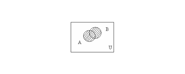
The union of the sets A and B is the set consisting of all those elements that belong to at least one of the sets A, B (Fig. 1.1): A ∪ B = {x | x ∈ A ∨ x ∈ B}.
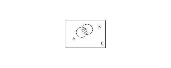
The intersection of sets A and B is the set consisting of all those and only those elements that belong simultaneously to both the set A and the set B (Fig. & 1.2): A ⋂ B = {x | x ∈ A ∧ x ∈ B}.
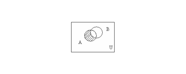
The difference between the sets A and B is the set of all those and only those elements A that are not contained in B (Fig. 1.3): A\B = {x | x ∈ A and x ∉ B},
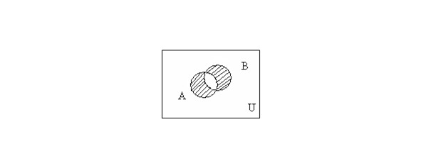
The symmetric difference of sets A and B is the set of elements of these sets that belong either to the set A or to the set B, but do not belong to their intersection (Fig. & 1. 4): A+B= {x | x ∈ A, or x ∈ B, x ∉ A⋂ B},
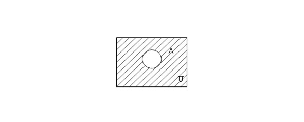
Absolute complement (negation) of the set A is the set of all those elements that do not belong to the set A (Fig. & 1. 5): ̅A=U\A,
1.4. Set Operations Properties
For arbitrary sets A, B, and C, the following relations are true.
Commutativity of the union: A ∪ B = B ∪ A,
Commutativity of the intersection: A ⋂ B = B ⋂ A,
Associativity of the union: A ∪ (B ∪ С) = (A ∪ B) ∪ С,
Associativity of the intersection: A ⋂ (B ⋂ С) = (A ⋂ B) ⋂ С,
Distribution of the union with respect to the intersection: A ∪ (B ⋂ С) = (A ∪ B) ⋂ (А ∪ С),
Distribution of intersection with respect to the union: A ⋂ (B ∪ С) = (A ⋂ B) ∪ (А ⋂ С),
Laws of action with empty and universal sets: A ∪ ∅ = A, A ∪ A = U, A ∪ U = U, A ⋂ U = A, A ⋂ A = ∅, A ⋂ ∅ = ∅
The law of idempotency of the union: A ∪ A = A,
The law of idempotency of the intersection: A ⋂ A = A,
De Morgan’s laws: A ∪ B = A ⋂ B, A ⋂ B = A ∪ B,
Laws of absorption: A ∪ (A ⋂ B) = A, A ⋂ (A ∪ B) = A,
Gluing laws: (A ⋂ B) ∪ (A ⋂ B) = A, (A ∪ B) ⋂ (A ∪ B) = A,
Poretsky Laws: A ∪ (A ⋂ B) = A ∪ B, A ⋂ (A ∪ B) = A ⋂ B,
Double Supplement Law A=A,
1.5. Euler-Venn Diagrams
The illustrations below are called Euler-Venn diagrams, they can be used to illustrate the equalities sets expressed through given sets, as well as receive new equalities.
1.6. Characteristic functions
1.6.1. Main relations
To prove complex set-theoretic identities, it is more efficient to use characteristic functions.
A characteristic function XA of the set A ⊆ U is a function defined on the set U with values on the set {0,1}: XA (x) = {1 if x ∈ A 0 if x ∉ A},
Obviously, the identity L = R will be valid if the characteristic functions of the sets L, Rare equal, i.e.. XL (x) = XR (x).
We give the characteristic functions of intersection, union, difference, absolute complement and symmetric difference, as well as an important property of the characteristic functions:
— XA ⋂ B (x) = XA (x) *XB (x)
— XA ∪ B (x) = XA (x) +XB (x) — XA (x) *XB (x)
— XA \ B (x) = XA (x) — XA (x) *XB (x)
— XA (x) = 1 — XA (x)
— XA + B (x) = XA (x) +XB (x) — 2XA (x) XB (x)
— XA (x) = X2A (x)
1.6.2. The process of evidence by the characteristic function
To prove the validity of the set-theoretic identities should express the characteristic features of its left and right sides of the characteristic features contained in them sets.
As an example, we prove the validity of one of the laws of action with an empty set: A ⋂ A = ∅.
Using the characteristic functions: XA ⋂ B (x) = XA (x) *XB (x), XA (x) = 1 — XA (x), we obtain: XA ⋂ A (x) = XA (x) *XA (x) = XA (x) * (1 — XA (x)) = XA (x) — X2A (x) =0
WHAT AND NEEDED TO BE PROVEN.
1.7. Relationships
Relationship is a mathematical structure that formally defines the properties of various objects and their relationships. Relations are usually classified by the number of objects to be linked and their own properties.
An ordered pair (x,y) is intuitively defined as a collection consisting of two elements x and yarranged in a specific order. Two pairs (x,y), (u,v) are considered equal if x=u, y=v and only if. The ordered n-th elements x1,…,xn are denoted by (x1,…,xn).
The Cartesian product of the sets X and Y is the set X × Y of all ordered pairs (x, y) such that x ∈ X, y ∈ Y.
A binary (or two-place) relation R is the set of ordered pairs, a binary relation is a subset of the Cartesian product.
If R is a relation and the pair (x, y) belongs to this relation, then along with the record (x, y) R, the notationis also used xRy. Elements x and y are called the coordinates (or components) of the ratio R.
The domain of a binary relation R is the set DR= {x ∨ ∃ y, xRy}. The range of binary relations R is the set ER= {y ∨ ∃ x, xRy}.
Let R XY be defined in accordance with the image in Figure 1.6
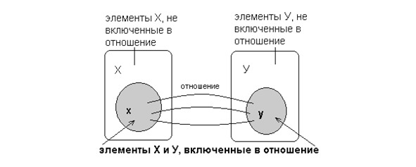
The domain of definition of DR and the range of values of ER are defined respectively: DR= {x: (x, y) ∈ R}, ER= {y: (x, y) ∈ R}. The binary relation can be set in any of the ways job sets. In addition, relations defined on finite sets are usually specified: by a
— list (enumeration) of pairs for which this relation is satisfied;
— matrix — the binary relation corresponds to a square matrix of order n, in which the element rij, standing at the intersection of the i-th row and the j-th column, is 1 if ai and aj is the relation, or 0 if it is absent: R= rij, rij= [0, (ai, aj) ∉ R 1, (ai, aj) ∈ R]
1.7.1. Properties of binary relations
— relationship R on the set X is reflexive if for any element xX hRh performed.
— The ratio R for the set X is called anti-reflective (irreflexive) if for any element xX performed ¬ (xRx).
— The ratio R for the set X is symmetric if for all x,x from hRu should be uRh.
— The ratio R for the set X is antisymmetric if for all x, yX of hRu and that x=y.
— A relation R on a set X is called transitive if, for any x, y, z X from xRy, and xRz follows yRz.
A partial order relation R is called linear order if the condition ∀x, y ∈ X: xRy ∨ yRx is satisfied.
A relation R is called a strict order relation on a set Xif it is antireflexive, antisymmetric, and transitive.
Reflective, symmetric, transitive relation on a set X is an equivalence relation on the set X.
Reflexive transitive and antisymmetric ratio is called a partial order relation, or the ratio of the non-strict order on the set X.
If theon the set X relation of partial orderis given ≤, then the set X is called partially ordered. If theon the set X relation of linear orderis given ≤, then the set X is called linearly ordered. If aon a set X relation of full orderis given ≤, then the set X is said to be completely ordered.
Let R — equivalence relation on the set X.
An equivalence class generated by an element x ∈ X is a subset of the set Xconsisting of those elements y X for which xRy. It is designated as: [x] = {y ∈ X | xRy}.
A partition of a set X is a collection of pairwise disjoint subsets of Xsuch that each element of the set X belongs to one and only one of these subsets.
Examples:
1. X= {1,2,3,4,5} Partition: {{1,2}, {3,5}, {4}}.
2. The partition of many students of the institute can be a set of groups.
In other words, a partition of a set X is a family: X = ∪i ∈ IXi∀i, j Xi ⋂ Xj j =0, Xi ⊆ X is an element of the partition.
The set of equivalence classes of elements of any set of X by the equivalence relation R setis the quotient of the set X with respect R denotedand X/R.For example, a plurality of student groups of a given university is a factor in a plurality of a plurality of university students in relation to belonging to one group.
Examples:
— (x, ≤) x ≤ y (x,y) ∈ ≤ — are comparable;
— (x,y) ∉ ≤ — are not comparable.
If (x, ≤), ∀ x ∈ X ∃ a ∈ X ∨ a ≤ x then a is the smallest element. If ∃ a ∈ X ∨ ∀ x ∈ X x ≤ a, then a is the largest element.
Statement: the largest or smallest element is single.
Proof: let a and b be the largest elements in (x, ≤), then ∀ x ∈ X a ≥ x, in particular a ≥ b. Similar to b ≥ a, therefore a=b.
In a similar way, the statement for the smallest elements is proved.
APPROVED PROVEN
1.7.2. Operations on binary relations
Since relations on X are defined by subsets R ⊆ X × Y, the same operations are defined for them as on sets.
— The union R1 ∪ R2: R1 ∪ R2= {(x,y) | (x,y) ∈ R1 or (x,y) ∈ R2}
— Intersection R1 ⋂ R2: R1 ⋂ R2= {(x,y) | (x,y) ∈ R1 and (x,y) ∉ R2}
— Difference R1/R2: R1/R2= {(x,y) | (x,y) ∈ R1 and (x,y) ∉ R2}
— Addition R: R=U/R, where U=M1×M2 (or U=M2)
The inverse ratio R-1:x R-1y if and only if yRx, R-1= {(x,y) ∨ (y,x) ∈ R}.
Compound ratio (composition) R1 ∝ R2. Let the sets M1, M2 and M3 and the relationship R1M1M2 and R2M2M3. The composite relation acts from M1 to M2 by means of R1, and then from M2 to M3 by R2, i.e. (a,b) R1 ∝ R2, if there is such an M2 that (a,c) R1 and (a,c) R2.
The transitive closure of R.A transitive closure consists of such and only such pairs of elements a and b from M, that is, (a, b) R, for which in M there exists a chain of (k +2) elements M, k 0 such that a, c1, c2, … ck, b, between whose adjacent elementsis fulfilled R. In other words, ARC1, with1RC2, …, withkRb.
Two partially ordered sets are called isomorphic if there is a one-to-one correspondence between them that preserves order.
Example: (x, ≤1), (y, ≤2) x, y are isomorphic if, where ∃φ:X → Y is a bijective function that preserves order (the definition of a function and a bijective function is given below).
A binary relation is called tolerance if it is reflective and symmetrical. A binary relation is called a quasiorder if it is irreflexive, antisymmetric, and transitive (preorder).
1.8. Functions
A binary relation f is called a function if from (x. y) f and (x. z) f it follows that y=z. Since functions are binary relations, the two functions f and g are equal if they consist of the same elements. The domain of the function is denoted by Df, and the domain is Rf. They are defined in the same way as for binary relations.
If f is a function, then instead of (x. y) f they write y=f (x) and say that y is the value corresponding to the argument x, or y is the image of the element x under the mapping f. Moreover, x is called the inverse image of the element y.
The concept of «display» is also often used. Display is some function that reflects the interconnection of elements between sets. In other words, the concepts of «function» and «display» are equivalent.
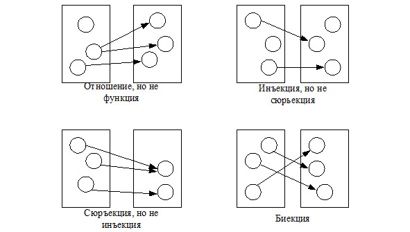
Let f: XY. A function f is called injective (injection) if: ∀x1,x2,y: {x1fyx2fy⇒x1=x2},
That is, each value of the function corresponds to a single value of the argument. A function f is called surjective (surjection) if ∀ y ∃ x | xfy. A function f is called bijective (bijection) if f is both surjective and injective.
Figure 1.7 illustrates the concepts of relationship, function, injection, surjection, and bijection.
1.9. Algebraic operations
An algebraic operation on a set M is a function φ: Mn → M, for n = 1 — unary operation, n = 2 — binary, n = 3 — triary (ternary).
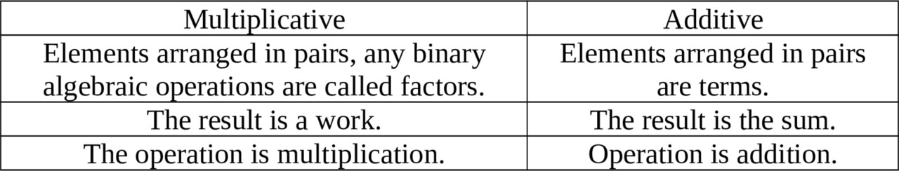
It is said thaton M a binary algebraic operation is definedif, by anyany ordered pair of elements of the set M. law, a well-defined element of the same set is associated withFor functions, multiplicative and additive terminology is used.
Properties:
— commutativity: a+b=b+a, a*b=b*a,
— () Associativity: a+b+c=a (a*b) *c=a* (b*c),
— distributivity: (a+b) *c=a*c+b*c,
A neutral element e of the set M for a binary algebraic operation φ:M2 → M is an element: e ∈ M ∨ ∀ x ∈ M φ (x, e) = φ (e, x) = x,
Theorem: the neutral element is the only one.
Proof: suppose that in the set M there are two neutral elements e and e». Then ∀ x ∈ M the equalities hold: φ (x, e) = x and φ (e’, x) = x. Therefore, these equalities hold for x=e’ and x=e: φ (e’, e) = e’ and φ (e’, e) = e, and it follows that e=e’.
THEOREM IS PROVEN.
1.10. Hasse diagrams
If x ≤ (precedes) y and x ≠ y, then write: x <(strictly precedes) y.
It is said that an element y covers an element xif x <y, and there is no element usuch that x <u <y. In the general case, if x <y, then either y covers x, or there exist elements x1, x2, …, xi, xi +1, …, xnsuch that x = x1 <x2 <… <xi <xi +1 <… <xn = y, where xi +1 covers xi for all i.
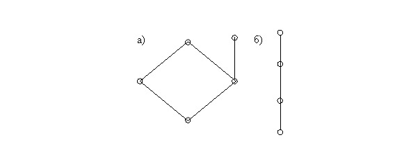
To illustrate the partial order on the set X, schemes are used that are called Hasse diagrams. In these diagrams, the elements of the set are represented as points on the plane. At the very bottom, the smallest element is depicted, if it exists and belongs to the set, or minimal elements, the elements covering the elements of the previous row, etc. are located higher, and if y covers x, then the points corresponding to them are connected by segments. Figure 1.8 shows the Hasse diagrams of two sets, and Figure 1.9b corresponds to a linearly ordered set.
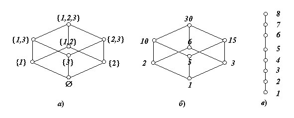
Let A = {1,2,3}. On the set 2,A = {∅, {1}, {2}, {3}, {1,2}, {1,3}, {2,3}, {1,2,3}}, we define the partial order relation «to be a subset», that is, x ≤ y if and only if when x ⊆ y. The Hasse diagram for this set is shown in Figure 1.9a.
Let X = {1,2,3,5,6,10,15,30}. On this set (divisors of 30), we define a partial order relation: x | y if and only if x divides y. The Hasse diagram for this set is shown in Figure 1.10.2b.
On a numerical set Y = {1,2,3,4,5,6,7,8} consider the relation ≤ (less than or equal to). The Hasse diagram for this set is shown in Figure 1.9c.
A Hasse diagram is a directed graph of the form: o→o→…→o→o
Consider the set of divisors of nordered by the divisibility relation. a/b ⇔ a divisor b (Dn,1),n ≥ 1,
Let p and q be prime integers greater than 1. We construct a Hasse diagram for which n=p2q.
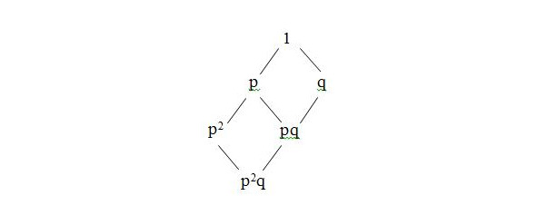
In the most general case, the Hasse diagram of a partially ordered set (Dn, 1) consists of edges of an n-dimensional parallelepiped, where n is the number of different prime divisors of n.
Theorem: n> 0, n=p1a1p2a2...pmam is the decomposition of the number n into the product of pairwise unequal simple factors. ∀ i,j (i≠j) ⇒ pi ≠ pj. The partially ordered set (Dn, 1) will be isomorphic to the Cartesian product of [a1] × [a2] × … × [am] linearly ordered sets.
Proof: we define an isomorphism as follows (by mapping into an m-dimensional cube): p1β1*p2β2*…*pmβm→ (β1,β2,β3,…,βm),
THEOREM IS PROVED.
1.11. Theorem
Two partially ordered sets X and Y Isomorphismare called isomorphic if there exists a bijection φ:X → Y that preserves a partial order relation. Otherwise: x1≤xx2 if and only if φ (x1) ≤yφ (x2), where ≤x is the partial order relation on the set X, and ≤y is the partial order relation on the set Y.
Statement: every partially ordered set X is isomorphic to some system of subsets of the set X partially ordered by the inclusion relation.
1.12. Algebraic structure
Everywhere defined (total function) φ: MnM→ called n-ary (n-place) operation on M.The set M together with the set of operations ∑= (φ1, φ2,…φm), φi: Mn→M, where ni is the arity of the operation φi, is called an algebraic structure, a universal algebra, or simply an algebra.
The set M is called the support or basis of algebra. The arity vector of operations (n1,n2,…,nm) is called the type of algebra. The set ∑ is called a signature.
A subset X of the set M (X ⊂ M) is said to be closed under the operation φif: ∀x1,x2,…,xn ∈ X φ (x1,x2,…,xn) ∈ X, (1.12.1)
If the set X is closed ∀ φ ∈ ∑, then X is called the support of another algebra: (X, ∑x) — and the set X together with the set of operations is called a subalgebra.
Theorem 1 (formulation 1): a nonempty intersection of subalgebras is also a subalgebra.
Proof: let (Xi, ∑ Xi) be the subalgebra (M; ∑). Then: ∀ i,j φiXi (x1,…,xn) ∈ Xi ⇒ ∀ j φjXi (x1,…,xn) ∈ ⋂ Xi, (1.12.2)
THEOREM IS PROVED.
Theorem 1 (formulation 2): the intersection of any system of subalgebras of the algebra G, if it is not empty, will be a subalgebra of this algebra.
Proof: indeed, if G takes a system of subalgebras Ai, i ∈ I, with non-empty intersection D and if ω ∈ Ωn, n≥1 and d1,d2,…,dn are any elements from D, then the element d1,d2,…,dnω contained in each of the subalgebras ai, and therefore is contained in D. On the other hand, in each of the subalgebras Ai, and therefore also in D, there are elements marked in G by all nullary operations from Ω. It follows that if M is a nonempty subset of the algebra G, then in G there exists a minimal among the subalgebras containing the whole set M, namely, the intersection of all such subalgebras. One of them is the algebraitself G.
THEOREM IS PROVEN.
The closure of the set X ⊂ M with respect to the signature ∑ (denoted by |X|∑) is the set of all elements (including the elementsthemselves X) that can be obtained from Xusing the operations from ∑. If the signature is implied, it can be omitted.
1.13. Theory
CategoryCategory Cis a pair (Obc, Homc (A,B)):
— set objects Obc;
— for each pair of objects A, B from the set of objects, a lot of morphisms (or arrows) are given Homc (A,B), and each morphism corresponds to unique A and B;
— for a pair of morphisms f ∈ Hom (A,B), g ∈ Hom (B,C) a composition is defined f o g ∈ Hom (A,C);
— for each object A, an identical morphism is given idA ∈ Hom (A,A);
moreover, two axioms are fulfilled: the
— composition operation is associative;
— identity morphism acts f o idA = idB o f = f trivially.
If φ o f = f o φ — then the morphism is called a homomorphism. A homomorphism, which is an injection, is called a monomorphism. A homomorphism that is surjection is called an epimorphism. A homomorphism, which is a bijection, is called an isomorphism.
If the supports of the algebra coincide, then the homomorphism is called an endomorphism, and the isomorphism is called an automorphism.
The most important role in category theory is played by the concept of a monoid (semigroup with unity). The monoid M can be described as a set M with two functions: μM × M → Mη,:1 → M, such that the following diagrams are commutative:
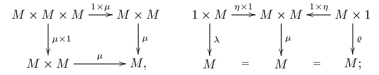
here 1 in the expression 1 × μ is the identical function M × M, and 1 in the expression 1 × M is a one-point set 1 = {0}, while λ ∧ ρ are bijections. The commutativity of the diagrams means that the following products coincide: μ o (1 × μ) = μ o (μ × 1), μ o (η × 1) = λ, μ o (1 × η) = ρ, (1.13.1)
Theorem: let two algebras be given: A= (A,∑A) and B= (B,∑B), then if f: A → B is an isomorphism, then f-1: B → A is also an isomorphism.
Proof: consider an arbitrary operation φ from signature A and the corresponding operation ψ from signature B.
We have: f (φ (a1,…,an)) =ψ (f (a1),…,f (an)), in addition, f is a bijection.
denote B1:= f (a1) …,bn:= f (a wherein a1 = f-1 (b1) …,an=f-1 ()
Then: f-1 (ψ (b1,…,bn)) =f-1 (ψ (f (a1),…,f (an))) =f-1 (f (φ (a1,…,an))) =φ (a1,…,an) =φ (f-1 (b1),…,f-1 (bn))
THEOREM IS PROVED.
If f: A → B is an isomorphism, then the algebras A and B are called isomorphic and are denoted as follows A~fB:
The isomorphism relation on the set of algebras of the same type is equivalent:
— reflexivity: A~fA, f:=I;
— symmetry: A~fB ⇒B~f-1A;
— transitivity: A~fB & B~gG⇒A~f o gG
1.14. Algebras with one operation (semigroups)
Semigroup — algebra with one associative operation: M= (M,o), (aob) oc=ao (boc),
Monoid is a semigroup with unit: ∃ e ∈ M| ∀x: e o x=x o e=x.
Theorem: the unit is the only one.
Proof: let: ∃ e1,e2 ∀a: a o e1=e1 o a= a & a o e2=e2 o a= a. Then: e1 o e2=e1 & e1 o e2 =e2 ⇒ e1=e2
THEOREM IS PROVEN.
A group is a monoid in which: ∀ a ∈ M ∃ a-1 ∈ M | a o a-1 = a-1 o a=e. The element a-1 is called the inverse. It is sometimes referred to as a».
Theorem: if thein the monoid for the element x opposite exists, then it is unique, that is, if x’*x=x*x’=e=x’«*x=x*x», then x’=x».
Proof: indeed, from the relations x*x»=e and x’*x=e it follows that: x’=x’*e=x’* (x*x») = (x’*x) *x»=e*x»=x».
THEOREM IS PROVEN.
Theorem: in the group the equationuniquely resolved a o x=b is.
Proof: let: a o x=b ⇒ a-1 o (aox) = a-1 o b ⇒ (a-1 o a) ox = a-1 o b ⇒ e o x = a-1 o b ⇒ x= a-1 o b.
THEOREM IS PROVEN.
A commutative group, that is, a group in which a o b = b o a is called Abelian. The following notation is used in abelian groups: a group operation is denoted by + or ⊕ the inverse of a: -a, the unit of the group denotes 0 and is called zero.
1.15. Algebra with two operations two operations
Let be given on a set: ⊗:M2→M is the multiplication and ⊕:M2→M is the addition. A ring is a set M with two binary operations ⊕ and ⊗, in which:
— addition is associative: (a ⊕ b) ⊕ c= a ⊕ (b ⊕ c)
— there is an addition unit: ∃0∈M∀aa⊕0=0⊕a=a
— there is an inverse addition element: ∀a∃-a,a⊕-a=0
— addition is commutative, that is, a ring is an Abelian addition group: a⊕b=b⊕a
— multiplication is associative, that is, a ring is a semigroup of multiplication: a ⊗ (b ⊗ c) = (a ⊗ b) ⊗ c the
— multiplication is distributive left and right: a ⊗ (b ⊕ c) = (a ⊗ b) ⊕ (a ⊗ c), (a ⊕ b) ⊗ c = (a ⊗ c) ⊕ (b ⊗ c) The ring is called commutative, if the multiplication is commutative: a ⊗ b = b ⊗ a. A commutative ring is called a unit ring if there is a unit of multiplication: ∃1∈Ma⊗1=1⊗a=a; that is, a ring with a unit is a monoid of multiplication.
1.16. Vector spaces
A field is a set M with two binary operations ⊕⊗ andsuch that:
— (a ⊕ b) ⊕ c= a ⊕ (b ⊕ c) — addition is associative;
— ∃0∈Ma⊕0=0⊕a=a — there is zero;
— ∀a∃-a | a⊕ (-a) =0 — there is an inverse element in addition;
— a ⊕ b = b ⊕ a — addition is commutative (field is an Abelian group by addition);
— a ⊗ (b ⊗ c) = (a ⊗ b) ⊗ c — multiplication is associative;
— ∃1∈M|a⊗1=1⊗a=a — there is a unit;
— ∀a ≠ 0∃a-1 | a-1⊗a=1 — there is an inverse element for multiplication;
— a ⊗ b = b ⊗ a — multiplication is commutative (field is an Abelian group by multiplication);
— a ⊗ (b ⊕ c) = (a ⊗ b) ⊕ (a ⊗ c) — Multiplication is distributive with respect to addition.
Let F= <F;+,.> be a field with the addition operation +, the operation of multiplication., the additive unit 0 and the multiplicative unit 1. Let V= <V;+,.> be some Abelian group with the operation + and the unit 0. If there exists an operation F × V → V (the sign of this operation is omitted) such that for any a,b ∈ F and for any x,y ∈ V the following relations hold: (a+b) →x=a→x⊕b→x;a (→x+→y) =a→x⊕a→y; (a*b) →x=a (b→x);1→x+x, then V is called the vector space over the field F, the elements of F are called scalar, the elements of V are called vectors, and the undefined operation F × V → V is called the multiplication of the vector by the scalar.
The unit of the group V is called →0 (zero-vector).
Theorem: ∀x∈V:0*→x=→0, ∀a∈F:a*→0=→0
Proof: (1—1) →x=1*→x-1*→x=→x-→x=→0
a (→0-→0) =a*→0-a*→0=→0-→0=→0
THEOREM IS PROVED.
1.17. Modular arithmetic
It is said that the number a is comparable modulo n with the number b (a=b (mod n)) if a and b divided by n give the same remainder: a=b (mod n) ⇔ a mod n=b mod n.
The comparability relation is reflexive, symmetric and transitive and is an equivalence relation. Equivalence classes with respect to comparability are called residues modulo n. The set of residues modulo n is denoted by zn. Over the residue modulo n, the operationsdefined +n, *n are: a+nb = (a+b) mod n, a*nb = (a*b) mod n,
It is easy to see that (zn, +n) is an Abelian group, and (zn, +n,*n) is a commutative semiring.
Numbers a and b are called coprime if their greatest common divisor is 1.
Let n — a positive integer, n ∈ N. φ (n) is the number of natural numbers 0 <a ≤ n coprime to n. n=10,d= {1,3,7,9}, φ (10) =4,
Function φ (n) is named after Euler. Assuming zn* ⊂ zn is the set of numbers coprime to n, we obtain that the Euler function φ (n) = |zn*|.
Let a natural number nbe presented, represented as its canonical decomposition into simple factors pi: n=k ∏ i=1= piai
Then the Euler function can be calculated by the formula: φ (n) =k ∏ i=1= piai-1 (pi-1)
It is assumed that φ (1) =1.
The Euler function can also be represented as the so-called Euler product: φ (n) =n ∏ p|n= (1- (1/p))
where p is a prime number and runs through all the values involved in the expansion of n into prime factors.
Euler’s theorem (ageneralization of Fermat’s small theorem): ∀a∈zn*,aφ (n) =1 (mod n)
1.18. Commutative semiring
A nonempty set S with the binary operationsdefined on it + and certain is called a commutative semiring if the following axioms hold.
— (S, +) is a commutative semigroup with neutral element 0, i.e.: ∀a,b∈S:a+b=b+a; ∀a,b,c∈S: (a+b) +c=a+ (b+c); ∃0∈S, ∀a∈S,0+a=a+0=a
— (S, *) is a commutative semigroup with neutral element 1, i.e.: ∀a,b∈S: ab=ba; ∀a,b,c∈S: (ab) c=a (bc); ∃1∈S, ∀a∈S,1a=a1=a
— Multiplication is distributive with respect to addition: ∀a,b,c∈S: a (b +c) =ab+ac, (a+b) c=ac+bc
— ∀a∈S:0a=a0=0
To construct the classical semiring of quotients, one can use the following method.
Consider a pair of non-negative integers (a,b),b ≠ 0.
We assume that the pairs (a, b) and (c, d) are equivalent, if ad = bc, we obtain a partition of the set of pairs into equivalence classes. Then we introduce operations on classes that turn the set of classes of equivalent pairs into a half-field that contains a semiring of non-negative numbers.
Weelement n ∈ S call anmultiplicatively reducible if ∀ a,b ∈ S from the equality an = bn that a = b. Denote by R the set of all multiplicatively reducible elements.
Statement: a multiplicatively reducible element is not a zero divisor.
Proof: Let s be a zero divisor, i.e. as = 0 for some a ≠ 0. Then as = 0s, but a ≠ 0 ⇒ is reducible not multiplicatively.
APPROVED PROVEN.
Let S — commutative semiring contractibly by elements of (s,r) ∈ S × R. Consider the set of ordered pairs of We introduce the relation ~ on S × R: (a,b) ~ (c,d) ⇔ ad=bc for all a,c ∈ S and b,d ∈ R.
Adoption: attitude ~ is an equivalence relation on S.
We show that ~ is an equivalence relation. To do this, it is necessary to show reflectivity, symmetry and transitivity.
Reflectivity: due to the commutativity of the semiring S: ab=ba ⇒ (a,b) ~ (a,b);
Symmetry: (a,b) ~ (c,d) ⇔ ad=bc ⇔ cb=da ⇔ (c,d) ~ (a,b);
Transitivity: (a,b) ~ (c,d) ⇔ ad=bc | × f ⇒ adf=bcf ⇒ afd=bcf
(c,d) ~ (e,f) ⇔ cf=de | × b ⇒ cfb=deb ⇒ bcf=bed
Consequently: afd=bed ⇒af =be ⇔ (a,b) ~ (e,f)
Thus, the ratio ~ is an equivalence relation on S.
APPROVED PROVEN
The semiring S is divided into equivalence classes; in each class are those elements that are in relation ~.
Denote by [a, b] the equivalence class of the pair (a, b). We introduce operations on the set Qcl (S) of all equivalence classes: [a,b] + [c,d] = [ad+bc, bd]
[a,b] * [c,d] = [ac, bd]
bd ∈ R since for n ∈ R,m ∈ R,a,b ∈ S, nma=nmb from here, since n ∈ R We obtain ma = mb, and since m ∈ R, then a = b, hence mn∈ R.
We show the correctness of the operations introduced.
Let: (a,b) ~ (a’,b’), (c,d) ~ (c’,d’)
Then (ad+bc) b’d’=adb’d’+bcb’d’=ab’dd’+cd’bb’=ab’dd’+c’dbb’=a’d’bd+c’d’bd= (a’d’+b’c’) bd ⇒ (ad+bc, bd) ~ (a’d’+b’c’,b’d’), (1.18.5)
acb’d’=ab’cd’=ba’dc’=bda’c’=a’c’bd ⇒ (ac, bd) ~ (a’c’, b’d’), (1.13.1)
Theorem: (Qcl (S),+,*) is a commutative semiring with 1,S ⊆ Qcl (S).
Evidence: to prove that the set Qcl (S) of all equivalence classes is a commutative semiring with 1, we need to show the closedness of operations on it.
— Addition. ∀ a,c,e ∈ S and ∀ b,d,f ∈ R: [a,b] + [c,d] = [ad+bc, bd] = [cb+da, db] = [c,d] + [a,b]; ([a,b] + [c,d]) + [e,f] = [ad+bc, bd] + [e,f] = [(ad+bc) f+bde, bdf] = [adf+bcf+bde, bdf]; [a,b] + ([c,d] + [e,f]) = [ab] + [cf+ de, df] = [adf+b (cf+de), bdf] = [adf+bdf+bde, bdf].
Since the right-hand sides are equal, the left-hand sides are also equal: ([a,b] + [c,d]) + [e,f] = [a,b] + ([c,d] + [e,f])
We show that ∀ n,n’ ∈ R: [0,n] = [0,n’]. Since 0n’ = n0 ⇔ (0,n) ~ (0,n’) ⇒ [0,n] = [0,n’]. The class [0, n] is neutral in +: [a,b] + [0,n] = [an, bn]
From the equality anb=bna ⇒ (an, bn) ~ (a,b) then [an, bn] = [a,b].
∀ n ∈ R [0,n] is a separate class playing thein Qcl (S) role of zero.
— Multiplication. ∀ a,c,e ∈ S and ∀ b,d,f ∈ R: [a,b] * [c,d] = [ac, bd] = [ca, db] = [c,d] * [a,b]; ([a,b] * [c,d]) * [e,f] = [ac, bd] * [e,f] = [ace, bdf]; [a,b] * ([c,d] * [e,f]) = [a,b] * [ce, df] = [ace, bdf].
From the equality of the right-hand sides it follows that: ([a,b] * [c,d]) * [e,f] = [a,b] * ([c,d] * [e,f])
Let us show that for ∀ n,n’ ∈ R [n,n] = [n’,n’]. Let nn’=nn’ ⇔ (n,n) ~ (n’,n’) ⇒ [n,n] = [n’,n’].
The class [n, n] is neutral in multiplication (a unit of a half ring), because [a,b] * [n.n] = [an, bn] = [a,b], since from the equality anb=bna ⇒ (an, bn) ~ (a,b); then [an, bn] = [a,b].
Multiplication is distributive with respect to addition: ([a,b] + [c,d]) * [e,f] = [ad+bc, bd] * [e,f] = (ade+bce, bdf]; [a,b] * [e,f] + [c,d] * [e,f] = [ae, bf] + [ce, df] = [aedf + bfce, bfdf] = [(ade + bce) f, (bfd) f] = [ade + bce, bfd] * [f,f] = [ade + bce, bfd]
Consequently, the right-hand distribution law holds:-hand distribution law is ([a,b] + [c,d]) * [e,f] = [a,b] * [e,f] + [c,d] * [e,f]
The leftproved in the same way.
THEOREM IS PROVEN
1.19. Group
Substitution on the set is the map of Zn = {1,2,…,n} into itself. Substitution: π = (1,2,…,n; i1,i2,…,in)
we will set the line (i1,i2,…,in).
A permutation is called cyclic (or a cycle) if some number j1 is translated by it into j2, j2 — by j3, etc., jk-1 is translated into jk, jk — by j1, and all the others the numbers remain in place. Such a cycle is denoted by (j1,j2,…,jk). The number k is called the cycle length. Arbitrary substitution can be represented as a product of cycles. For example: (1,2,3,4,5;2,1,4,5,3) = (1,2) (3,4,5)
A cycle of length 2 is called transposition.
Theorem: any substitution is representable as a product (i.e., sequential execution) of transpositions.
A substitution that can be represented as the product of an even (odd) number of transpositions is called even (respectively, odd).
Theorem: permutations on the set Zn form a group with respect to the product operation.
Proof: the operation of the product of permutations π1 and π2 consists in their sequential application. For example, if: π1= (1,2,3,4;2,4,3,1) π2= (1,2,3,4;1,4,3,2)
then: π1π2= (1,2,3,4;4,2,3,1)
The product operation has, as is easily verified, the associativity property: π (στ) = (πσ) τ The identity element of the group is the identity substitution: The (1,2,…,n;1,2,…,n)
substitution inverse to: (1,2,…,n;i1,i2,…,in)
is the substitution: ( i1,i2,…,in;1,2,…,n)
THEOREM IS PROVED.
Group permutations on the set Zn called symmetric group nth power, denoted by Sn.The number of elements of the symmetric group nth power is equal to n!.
If the substitution on the set Nn is represented as the product of b1 cycles of length 1, b2 cycles of length 2, etc., bn cycles of length n, then they say that the substitution is of the type: b1,b2,…,bn For example, wildcard: π1= (1,2,3,4;2,4,3,1)
has a type (1,0,1,0).
Let M and N be finite sets, and G and H be permutation groups onrespectively M and N,. Degreesgroup HG consists of all possible pairs of (π; σ),where the π ∈ G, σ ∈ H and acts on a plurality NM of all functions f:M → N.
Moreover, by definition (π;σ) f (x) =σf (π (x)) for all x ∈ M and f ∈ N M.
Functions f1 and f2 from NM are called equivalent (f1 ~ f2) if: ∃π | f1 (πx) = f2 (x) for all x ∈ M
1.20. Boolean functions
A Boolean function (either a logical function or a function of a logic algebra or a switching function) of n variables is a mapping: f:E2n → E2
where E2n = {0,1} Is a Boolean set.
Elements of the Boolean sets 1 and 0 are usually interpreted as logical values of «true» and «false», although in the general case they are considered as formal symbols that do not carry a certain meaning. A non-negative integer n is called the arity or locality of the function; in the case n = 0, the Boolean function turns into a Boolean constant. Elements of the Cartesian product are called Boolean vectors.
The set of all possible Boolean functions: Pn= {f|f:E2n → E2}
Each Boolean function of arity n is completely determined by setting its values on its domain of definition, that is, on all Boolean vectors of length n. It is easy to calculate the number of all Boolean functions of n variables.
Theorem:| Pn|=22n
Proof: Indeed, the number of functions from ak-element setAto anm-element setBis equal tomk (this fact is proved in the section on combinatorics). In our case, B = {0, 1}, andA = Bn. Thenm = 2 andk = |Bn| = 2n. This implies the statement of the theorem.
THEOREM IS PROVEN
Any Boolean function can be set by the truth table.
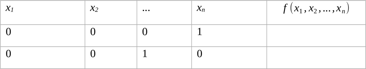
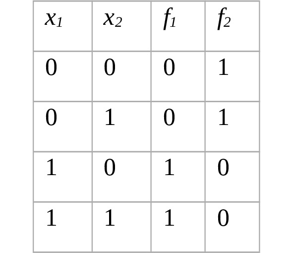
For these functions, x1 is essential and x2 Is an inconsequential variable. The variablevalue of functions x2 does not affect the, i.e. the value of the function does not significantly depend on the variable x2. f1=x1,f2= ¬ x1
Boolean functions are equal if one of the other is obtained by introducing or deleting non-essential variables.
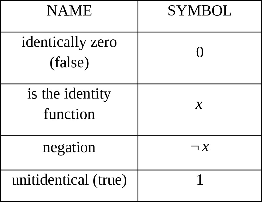
1.20.1. Boolean functions of one variable
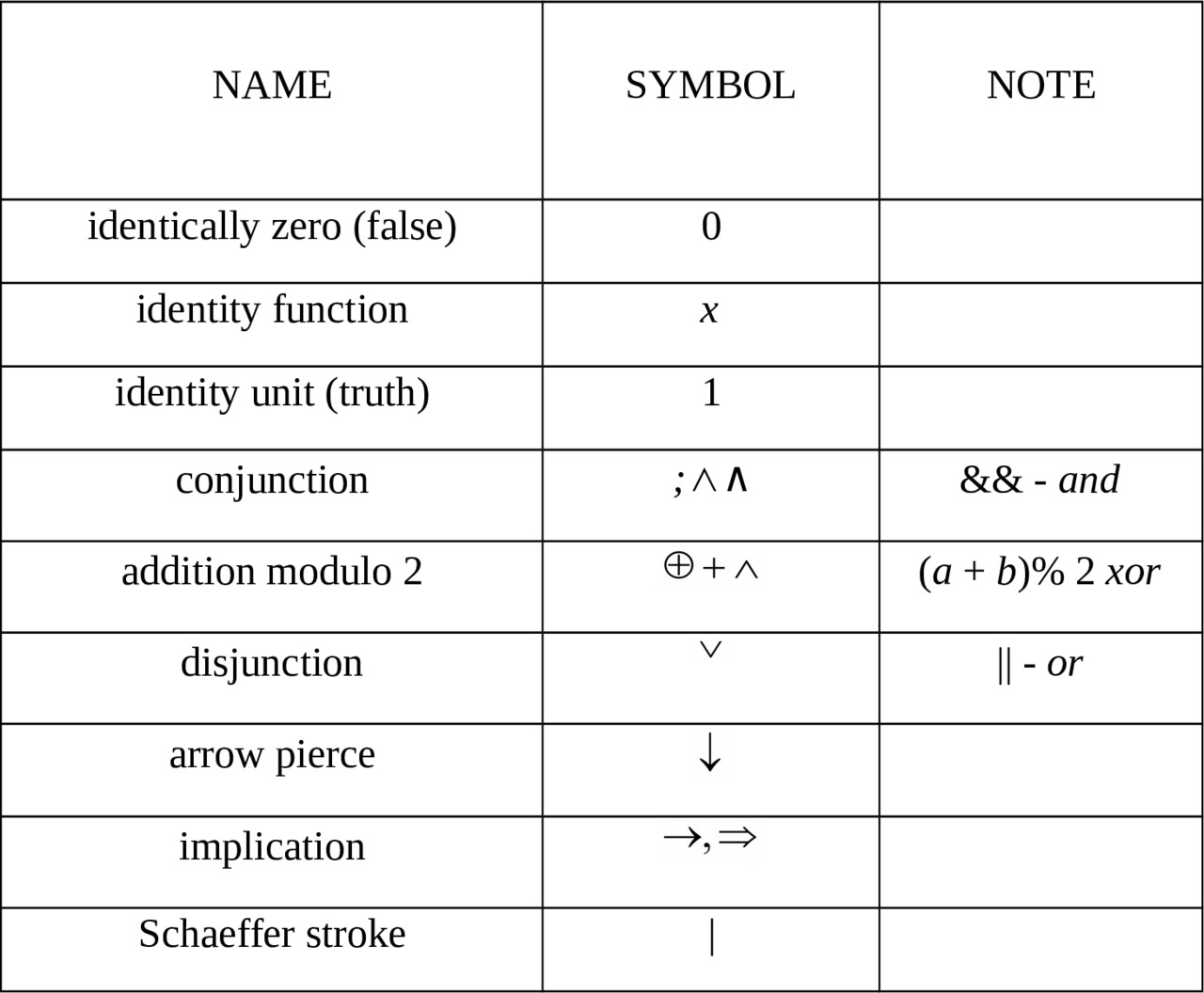
1.20.2. Boolean functions of two variables of
F= (f1,f2,…,fn), ∀ i: fi ∈ Pn
Formula over F: Ф [F] = fi (t1,t2,…,tm), fi ∈ F, ti — variable or formula. The set F is called a basis. The function fi is called an external (main) operation; ti is the subformula.
1.21. Equivalent formulas
Formulas are called equivalent if they implement the same function. In other words, two logical formulas are called equivalent if, for any values of their logical variables that are the same for both functions, these formulas take the same values. F1=F2:=func (F1) =f&func (F2) =f
Equivalent formulas serve to express some logical operations through others, simplify formulas or, more precisely, replace some logical formulas with others that are equivalent, but simpler. In reasoning one can replace complex statements with simpler ones equivalent to them.
A formula is called identically true or a tautology if it implements an identity unit.
A formula is called identically false if it implements an identity zero.
Statement: the equivalence relation of formulas is equivalence.
«Allequivalence can be checked by the relevant construction of the truth table STI.
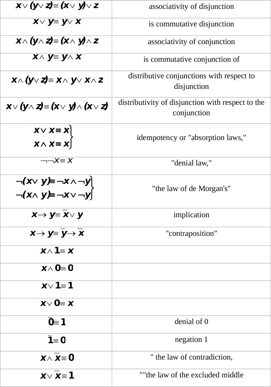
The set (E2, ¬, ∨, ∧) is called a binary Boolean algebra. In other words, 2 constants are defined on it: 1 and 0, and the operations of negation, conjunction and disjunction.
Substitution rule: if in the equivalent formulas instead of the same variable x we substitute the same formula, then we get equivalent formulas. ∀Г (Ф1 (…x…) =Ф2 (…x…)) Ф1 (…x…) {Г\\x} =Ф2 (…х…) {Г\\x}
In this case, the sign \\ we have designated the replacement of all occurrences of a variable with a formula. The condition for replacing all occurrences is essential.
Replacement rule: if in some formula we replace some subformula (we use the \ sign to replace) with an equivalent one, we get an equivalent formula. Ф (…Г…) ∨ Г1=Г2⇒ Ф (…Г…) {Г1\Г} =Ф (…Г…) {Г2\Г}
1.22. Algebra of Boolean functions
Define the conjunction, disjunction and negation functions: ∧, ∨: Pn2 → Pn; ¬: Pn → Pn
They are operations on the set of Boolean functions. The algebraic structure (Pn, ∨, ∧, ¬) is called the algebra of Boolean functions. The algebra of Boolean functions is a Boolean algebra. All axioms of Boolean algebra are satisfied in the algebra of Boolean functions.
Ф is the set of formulas equivalent to given ones; we denote K= {Ф} Ф is the equivalence class with respect to equivalence.
An algebra of the class of formulas (K, ¬, ∨, ∧) is called the Lindenbaum-Tarski algebra. This algebra is isomorphic to the algebra of Boolean functions and is a Boolean algebra.
1.23. The principle of duality
In Boolean algebras, there are dual statements; they are either true or false at the same time. Namely, if in a formula that is true in some Boolean algebra, change all conjunctions to disjunctions, 0 to 1, ≤ to ≥ and vice versa, then we get a formula that is also true in this Boolean algebra. f (x1,x2,…,xn) ∈ Pn
f (x1,x2,…,xn) = f (x1,x2,…,xn) is the dual function f.
Theorem: duality is foreign-valued: (f*) *=f
Proof: f* = f (x1,x2,…,xn)
(f*) *=f (x1,x2,…,xn) def= f (x1,x2,…,xn)
THEOREM IS PROVED.
A function is called self-dual if f*=f.
Theorem: let φ (x1,x2,…,xn) be realized by the formula:
f (f1 (x1,x2,…,xn),…,fn (x1,x2,…,xn))
then the formula :
f* (f1* (x1,x2,…,xn),…,fn* (x1,x2,…,xn))
implements the function:
φ (x1,x2,…,xn)
Proof: φ* (x1,…,xn) =φ (x1,…,xn) =φ (x1,…,xn) =f (f1 (x1,…,xn),…,fn (x1,…,xn)) =f (f1 (x1,…,xn),…,fn (x1,…,xn)) = f (f1* (x1,…,xn),…,fn* (x1,…,xn)) =f* (f1* (x1,…,xn),…,fn* (x1,…,xn))
THEOREM IS PROVEN.
Corollary: Ф1=Ф2⇒ Ф1*=Ф2*.
Further, proving a theorem, by the principle of duality we immediately get a dual theorem: x1 ∨ x2= x1 ∧ x2
x1 ∧ x2= x1 ∨ x2
By normal form we mean a syntactically unique way of writing a formula. We introduce a special kind of entry: xy=x ≡ y, if x = y, xy=1, if x ≠ y, xy=0
The decomposition theorem of a Boolean function can be represented as a disjunctive conjunction of conjunction: f (x1,x2,…,xm, xm+1,…,xn) =||= δ1, δ2,…,δmx1δ ∧ x2δ ∧…∧ xmδm ∧ f (δ1, δ2,…,δm, xm+1,…,xm)
where disjunctions are taken over all possible δ.
Proof: in order to prove that a given formula implements a function, it is enough to take an arbitrary set of argument values, calculate the values of formulas on this set and, if it turns out to be equal to the value of the function, then the formula really implements the function:
(δ1, δ2,…,δmx1δ ∧ …∧ xmδm ∧ f (δ1,…,δm, xm+1,…,xn)) (a1,a2,…,an) =δ1, δ2,…,δma1δ1 ∧ …∧ amδm ∧ f (δ1,…,δm, am+1,…,an) = aa1 ∧ a2a2 ∧ …∧ amam∧ f (a1,a2,…,an) = f (a1,a2,…,an)
THEOREM IS PROVED.
1.24. Perfect normal forms
All algebraic terms of a formula include all variables. It is said that a certain class of formulas K has a normal form if there is another class of formulas K», which are called normal forms, such that any formula of the class K has a unique equivalent formula from the class K»: ∃K! ∀Ф∈K∃!Г∈K»∨Ф=Г
1.24.1. Perfect Disjunctive Normal Form
Representation of a Boolean function in the form (a disjunction is a union sign):
f (x1,x2,…,xn) =δ1, δ2,…,δmx1δ1 ∧ x2δ2 ∧ …∧ xnδn
is called a perfect disjunctive normal form (SDNF).
Theorem: ∀f ∈Pn ∨ {0} ∃ the only representation in the form of SDNF.
Proof: we use the decomposition theorem for a Boolean function:
f (x1,x2,…,xn) =δ1, δ2,…,δnx1δ1 ∧ …∧ xnδn ∧ f (δ1,…,δn)) =f (δ1, δ2,…,δn) =1x1δ ∧ …∧ xnδn ∧ f (δ1,…,δn)) =f (δ1, δ2,…,δn) =1x1δ ∧ …∧ xnδn
THEOREM IS PROVED.
Theorem: every Boolean function can be expressed in terms of disjunction, conjunction and negation: ∀f ∈Pn∃Ф {¬, ∨, ∧} |funcФ=f
Proof:0=x ∧ x. In other cases, see the theorem above.
THEOREM IS PROVEN.
1.24.2. Perfect conjunctive normal forms
Theorem: every Boolean function can be represented in the form:
f (x1,…,xn) =f (δ1, …,δ2) =1x1δ ∨ … ∨ xnδn
Proof: by the duality principle from the SDNF theorem, it can be argued that every Boolean function has an SKNF.
Q.E.D.
1.25. Closed classes of Boolean functions
Let F be the set of Boolean functions: F= {f1,f2,…,fn},∀ifi∈ Pn
The closure of the set F is the set of Boolean functions realized by formulas over F: [F] = {f∈ Pn | f=func Ф [F]}
We introduce a special type of classes of Boolean functions.
— T0= {f|f (0,0,…,0) =0} — a class of functions that preserves 0;
— T1= {f|f (1,1,…,1) =1} — a class of functions that preserves 1;
— T*= {f|f =f*} is the class of self-dual functions;
— T≤= {f|α≤β⇒f (α) ≤f (β),α= (α1,α2,…,αn),β= (β1,β2,…,βn) ∀iai, bi∈ E2,α≤β ⇔ ∀iai ≤ bi is the class of monotonic functions;
— TL= {f|f=x0+C1x1+C2x2+…+Cnxn} is the class of linear functions.
Theorem: classes: T0,T1,T*,T≤,TL — closed.
Proof: in order to prove that some class is closed, it is enough to prove that if a function is implemented as a formula over this class, then it belongs to this class. The proof of the isolation of classes 4 and 5 is provided to readers as an exercise.
It can be proved that an arbitrary formula has this property by induction on the structure of formulas. The basis of each such induction is obvious. Functions from F are realized as trivial formulas over F. Thus, only inductive transitions need to be proved.
f0,f1,…,fn ∈ T0, Ф= f0 (f1 (x1,…,xn),…, fn (x1,…,xn)) = f0 (0,…,0) =0 ⇒ Ф ∈ T0
f0,f1,…,fn ∈ T1,, Ф= f0 (f1 (x1,…,xn),…, fn (x1,…,xn)) = f0 (1,…,1) =1 ⇒ Ф ∈ T1
f0,f1,…,fn ∈ T*,, Ф*= f0* (f1* (x1,…,xn),…, fn* (x1,…,xn)) = f0 (f1 (x1,…,xn),…, fn (x1,…,xn)) ⇒ Ф* ∈ T*,,
Q.E.D.
1.26. Completeness of a system of Boolean functions
As already mentioned, a Booleanis an arbitrary n-function place function f (x1,x2,…,xn), where xi ∈ {0,1}. The complete system of Boolean functions is denoted by E and has the following form: f1 (x1,x2,…,xk1) f2 (x1,x2,…,xk2) … fe (x1,x2,…,xke)
A system of functions Eis called complete if any of its Boolean functions can be expressed using f1, f2, … fe through superposition.
A superposition is a function f*, which is obtained from a function f using the following transformations:
— change of variable: f (x1,x2, xj, …,xn) f* = f (x1,x2, xj-1,y, xj+1, …,xn);
— substitution instead of xj of some function from the system.
f* = fi (x1,x2, xj-1, fe (x1,x2,…,xke),xj+1, …,xki)
Example: system of functions {¬, ∪, ⋂} =E1 is always complete, because each function of this system can be represented as SDNF, therefore, SDNF is a superposition through which any of the functions of the system can be expressed.
Example: the system of functions {¬, ∪} =E2 is also complete, since the missing function ∩ can be expressed in terms of the other two by the de Morgan rule and double negation:
x1 ⋂ x2= ¬ (¬ x1 ∪ ¬ x2)
Example: prove the completeness of the system: X → Y,0.
For clarity, this system can be written as follows: {→,0}. That is, we are given a system consisting of a Boolean function (implication) and a constant 0. With their help we can express the negation operation, for this we substitute the constant 0 instead of one of the variables:
X → 0= ¬ X ∪ 0 = ¬ X
Therefore, this system is complete.
Consider alternative definitions.
The set of Boolean functions of B= {f 1, f2,fm,…,…} is called a full system if any Boolean function can be implemented by the formula above B.
Theorem (on completeness): let two systems of functions frombe given P2: B1= {f1,f2,…} and B2= {g1,g2,…}. Then, if the system B1 is complete and each of its functions can be realized by a formula over B2, then the system B2 is also complete.
Proof: let h be an arbitrary function from P2. We show that it can be realized by the formula over B2.
Due to the completeness of B1 h is realized by the formula over B1, i.e. h= [ff1,f2,…]. In addition, by condition f1,f2,… are realized by formulas over B2, i.e. fi=Фi [g1,g2,…]. Therefore, in the formula Ф we can exclude the occurrence of symbols of functions f1,f2,…, replacing them with the corresponding formulas: Ф [Ф1 [g1,g2,…], Ф2 [g1,g2,…],…], (1.26.5)
The resulting expression defines a formula over B2that implements h.
THEOREM IS PROVEN
Example: the system {x,x ∧ y} is complete. Indeed, consider the systems B1= {x,x ∧ y, x ∨ y} and B2= {x,x ∧ y}. The system B1 is complete and, since x ∨ y= x ∧ y, then each function of this system is expressed by a formula over B2. Thus, the conditions of the completeness theorem are satisfied and, therefore, the system B2= {x,x ∧ y} is a complete system.
Example: the system {x|y} is complete. Indeed, consider the systems B1= {x,x ∧ y} and B2= {x|y}. We have: x|y= x ∨ y =xy. Therefore:
x|x=xx=x and xy=x|y= (y) | (x|y), (1.26.6)
Thus, each function of the system B1 is realized by a formula over B2. In addition, system B1 is complete. Therefore, the conditions of the completeness theorem are fulfilled and, therefore, B2= {x|y} is a complete system.
2. COMBINATORY
2.1. The basic principles of combinatorics
Theorem (principle of multiplication): if some action can be performed in k stages, and the number of possible ways of i-thstage is equal to ni (i=1,2,…,k),then the total number Nk of all possible ways of performing said action is calculated according to the formula:
Nk=n1*n2*…*nk=∏i=1kni, (2.1.1)
Proof: we use induction on the number of stages. If k = 1 then, obviously, N1 = n1 and, therefore, formula (2.1.1) is valid for k = 1.
Further, let k = 2. Then, since each of the n1 methods for implementing the first stage can take place with each of the n2 methods for implementing the second stage, then N2=n1*n2, i.e. formula (2.1.1) is also valid for k = 2.
Now suppose that formula (2.1.1) is valid for k = m — 1, i.e. the formula holds:
Nm-1=∏i=1m-1ni, (2.1.2)
Then, if k = m then, considering the first m — 1 stages as the first stage with the total number of implementation methods defined by the formula (2.1.2), and applying a result similar to the second step of induction, we obtain:
Nm=Nm-1*nm=∏i=1mni,
i.e. formula (2.1.1) is also valid for k = m.
THEOREM IS PROVEN.
Theorem: the number of elements of the Cartesian product is equal to the product of the numbers of the elements of the set participating in this Cartesian product:
|X×Y|=|X|*|Y|
Proof: Consider an action consisting of 2 stages. The first stage is the choice of the 1st element of an ordered pair. The second stage — the choice of the 2nd element of an ordered pair.
Then the 1st stage can be completed in |X| steps, the 2nd stage in |Y| steps. By the principle of multiplication,
THEOREM IS PROVED.
Theorem: the number of all possible functions from M to N, where the number of elements |M|=n, the number of elements |N|=m, is mn.
Proof: the first element from the set M can be mapped to m elements, the second element from the set M can be mapped to m elements, the third n etc. We get: m*m*…*m=∏i=1nmi=mn, where ∀i mi = m.
THEOREM IS PROVEN.
Theorem (addition principle): if object a can be obtained in n ways, object b — in m ways, then object «a or b» can be obtained in n + m — k ways, where k is the number of repeated methods. Set theoretic wording. If A ⋂ B ≠ ∅,then| ∪ || || || AB=A+B-A ⋂ |
Lemma: If A ⋂ B=∅,then |A ⋂ B|= 0,then |A ∪ |=|A|+|B|B.
Proof of the lemma: let A and B be finite sets such that A ⋂ B=∅, |A|=m, |B|=n. If the element a ∈ A can be selected in m ways, and the element b ∈ B — n ways, then the elementselected in x ∈ A ∪ B can be m + n ways. Let X1,X2,…,Xk be pairwise disjoint sets, Xi ⋂ Xj =∅, where i ≠ j. Then, obviously, the equality holds:
| ∪i=1kXi|= ∑i=1k|Xi|
The lemma is proved.
Proof of the principle: if we consider the union of two sets A and B, then we will not change anything if we consider a union of this kind:
A ∪ B=A ∪ (B\A)
It can be opened:
A ∪ B=A ∪ (B ⋂ A)
Now the number of union elements is:
|A ∪ B|=|A ∪ (B\A) |
Next we consider A ⋂ (B\A), which is equal to ∅. Accordingly, you can open the difference of the sets:
A ⋂ B ⋂ A= ∅ ⋂ B= ∅
We have the intersection of two sets, it is empty and there are the number of elements combining these sets. We use the lemma. We get:
|A ∪ B|=|A| + |B\A|
Further we consider the set B, it is:
B= (A ⋂ B) ∪ (B\A)
Moreover, if we take the intersection of these sets, we get:
(A ⋂ B) ⋂ (B\A) = ∅
Once again we return to the lemma and get: |B|= |A ⋂ B| ∪ |B\A|. Let us express from here: |B\A|, |B\A|= |B| — |A ⋂ B|
Substitute it in: |A ∪ B| =|A ∪ (B\A) | and get: |A ∪ B| =|A| + |B| — |A ⋂ B|
PRINCIPLE PROVED.
2.2. Placements
A placement with repetitions is the function f: {x1,x2,…,xm} → {y1,y2,…,yn}. Elements xi are called objects, and yj — drawers.
Placements with repetitions — combinatorial compounds made up of n elements of m. Moreover, each of the n elements may be contained as many times as desired or absent altogether.
Theorem: the number of all arrangements with repetitions is equal to the number of sequences {a1,a2,…,am} of numbers 1 ≤ ai ≤ n and, therefore, it is equal to nm.
Non-repetitive placements are combinatorial compounds made up of n elements of m each. In this case, two compounds are considered different if they either differ from each other by at least one element, or consist of the same elements, but located in different order.
Theorem: the number of placements without repetition is:
Anm= ((n!) / (nm)!)
Proof: the first item can be placed in n ways, the second — (n — 1), ⋅⋅⋅, mth- (n — m +1). We get: Anm=n (n-1) … (n-m+1) = ((n!) / (nm)!)
THEOREM IS PROVEN.
2.3. Combinations
Of a combination of elements of the set X is a subset of a finite set A ⊆ X. If |A|=k,|X|=n, then the subset A is called a combination of n in k, denoted by: Cnk. For example, combinations of the three colors of a seven-color rainbow will be described by subsets of three elements.
The combination can be interpreted as the placement of indistinguishable objects. Combinations are a k-element subset of a given set.
Theorem: the number of combinations of n over k is equal to:
Cnk= ((n!) / (k! (nk)!))
Proof 1: from the formulas: Akn=Ckn*k! and Ank= ((n!) / ((nk)!) — we get the necessary formula.
THEOREM IS PROVEN.
Proof 2: we consider an action consisting of two stages.
Stage I: n1=Cnk-1
Stage II: n2= (n-k+1) / (k), Cnk=Cnk-1* ((n-k+1) / (k))
Using this formula, we get: Cnk= ((n!) / (k! (nk)!))
THEOREM IS PROVEN.
Property 1: Cnk= Cn-1k-1+ Cn-2k-1 +…+Ck-1k-1
Proof (by induction): for n = 1, the induction basis holds.
For n = n +1: Cn+1k=Cnk-1+Cnk
Cn+1k=Cnk-1+Cn-1k-1+Cn-2k-1 +…+Ck-1k-1
((n+1)!) / (k! (n+1-k)!) = (n!) / ((k-1)! ((n-k+1)!)) + (n!) / (k! (n-k)!)
(n!* (n+1)!) / ((k-1)!*k (n-k)!* (n-k+1)) = (n!) / ((k-1)! (n-k)!* (n-k+1)) + (n!) / ((k-1)!*k (n-k)!)
(n+1) / (k (n-k+1)) = (1) / (n-k+1) + (1) / (k)
(n+1) / (k (n-k+1)) = (k+n-k+1) / (k* (n-k+1))
1 = 1 (true). Thus, the statement is true for any n.
PROPERTY PROVED
Proof (combinatorial):
Cnk=Cn-1k-1+Cn-2k-1 +…+Ckk-1+ CK-1k-1
Cn+1k=Cnk-1+Cnk
Cn-1k=Cn-1k-1+Cn-1k
Cn-1k=Cn-2k-1+Cn-2k
Cn-2k=Cn-3k-1+Cn-3k
…
Ck+1k=Ckk-1+Ckk
PROPERTY PROVED.
Property 2: Cnk=Cn-1k+Cn-1k-1
Proof:
((n-1)!) / (k! (n-1-k)!) + ((n-1)!) / ((k-1)! ((n-1-k+1)!)) = ((n-1)!) / (k! (n-1-k)!) + ((n-1)!) / ((n-1)! (n-k)!)) = ((n-1)! (n-k)) / (k! (n-k)!) + ((n-1)!k) / (k! (n-k)!) = ((n-1)! (n-k+k)) / (k! (n-k)!) + (n!) / (k! (n-k)!)
PROPERTY IS PROVED.
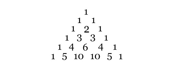
Property 3: Blaise Pascal suggested to consider and illustrate the properties associated with binomial coefficients, consider the Pascal triangle.
Theorem:∑k=0n Cnk=2n
Proof (combinatorial): on the left side of the equality is the number of all possible subsets of the set — by the Boolean theorem this number is 2n.
THEOREM IS PROVEN
Proof (by induction):
— For k = 0: ∑k=00 C0k=C00=1=20 the ⇒ equality is true.
— Assume that the equality holds for k = n, we prove the equality for k = n +1, i.e. we prove the equality: ∑k=0n+1 Cn+1k=2n+1=2* ∑k=0nCnk, or: Cn+10+Cn+11+Cn+12+Cn+13+…+Cn+1n-1+Cn+1n+Cn+1n+1=2 (Cn0+Cn1+Cn2+Cnn-2+Cnn-1+Cnn), (2.3.1)
To prove equality (2.3.1), we use: Cn+1k=Cnk-1+Cnk, (2.3.2)
Let us prove this equality: (n! (N+1)) / (k! (nk)! (n-k+1)) = (n!k) / (k! (nk)! (n-k+1)) + (n!) / (k! (nk)!)
(n+1) / (n-k+1) = (k) / (n-k+1) +1 ⇔ (n+1) / (n-k+1) = (n+1) / (n-k+1) the ⇒ equality (2.3.2) is proved. We return to the proof of (2.3.1): using equality (2.3.2) we obtain that: Cn+11=Cn0+Cn1;Cn+12=Cn1+Cn2
…
Cn+1n-1=Cnn-2+Cnn-1;Cn+1n=Cnn-1+Cnn
i.e. equality (2.3.1) takes the form: Cn+10+Cn+1n+1=Cn0+Cnn;1+1=1+1⇒
THEOREM IS PROVED.
Property 4: Cmn=Cmmn is the symmetry of the Pascal triangle.
Proof: (m!) / (n! (m-n)!) = (m!) / ((m-n)! (m-m+n)!)
PROPERTY PROVED.
Property 5: CniCim=CnmCnmim
Proof: (n!) / (i! (n-i)!) * (i!) / (m! (i-m)!) = (n!) / (m! (n-m)!) * ((n-m)!) / ((i-m)! (n-m-i+m)!)
PROPERTY PROVED.
Suppose there are objects of n different kinds, and from them are made up sets containing k elements. Such samples are called repeat combinations. Their number is denoted by Cnk.
Theorem: The number of combinations with repetitions can be calculated by the formula: Cmn=Cn+m-1n= ((n+m-1)!) / (n! (m-1)!), (2.3.3)
Example (cake problem): let it be required in the store to buy 7 cakes. The store has cakes of one of the types: eclairs, sand, puff, Napoleon. How many choices?
With each purchase we put in correspondence a sequence consisting of seven units and three delimiters 0. A total of 4 types of cakes, then zeros — 3.
Summarize the previous problem. The number of purchase options is equal to the number of permutations of n type I elements (units (cakes)) and m type II objects (zeros (delimiters)). Thus, rearranging by all means n units and (m — 1) zeros, we get the desired number:
P (n,m-1) = ((n+m-1)!) / (n! (m-1)!) =Cmn
The solution to the generalized purchase problem is a proof of (2.3.3).
2.4. Number of permutations
Letbe given n1 elements of the first type, n2 — the second type, …, nk — thek-th type, total n elements. Ways to place them in n different places are called repetitive permutations. Their number is denoted by:
Pn (n1,n2,…,nk)
Theorem: the number of permutations without repetition is:
Pn (k1,k2,…,km) = (n!) / (k1!k2!…,km!)
Proof: a subset of A1 can be chosen Cnk1 in ways. A subset of A2 is selected from the remaining (n — k1) elements, it can be selected in Cn-k1k2 ways. A subset of A3 — Cn-k1-k2k3 ways, etc. Select a subset Am defined by previous subsets. From here we get: P(k1,k2,...,km)=Cnk1Cn-k1k2...Cn-k1-… -km-2km-1= (n!) / (k1! (n-k1)!) * ((n-k1)!) / (k2! (n-k1-k2)!) … ((n-k1-… -km-2)!) / (km-1! (n-k1-… -km-2-km-1)!)
Since n-k1-… -km-1= km, then after reducing the fraction we get the desired equality.
THEOREM IS PROVEN.
The number of one-to-one functions, or the number of permutations of n objects, is denoted by P (n).
Theorem: the number of permutations of elements is n! or n elements can be rearranged n! way, i.e. P (n) =n!
Proof: we can put the first item in one of n positions, the second in (n — 1), etc., the last item can only be put in one place, and this is the definition of n!:
P (n) =Ann=n* (n-1) *…* (n-n+1) =n* (n-1) *…*1=n!, (2.4.4)
THEOREM IS PROVED.
Comment. Fair recurrence formula: P (n) =n*Pn-1
2.5. Inclusion and exclusion formula (main theorem)
The formulas and algorithms given in the previous sections give methods for calculating combinatorial numbers for some common combinatorial configurations. Practical tasks are not always directly reduced to known combinatorial configurations. In this case, various methods are used to reduce some combinatorial configurations to others.
Consider the principle of inclusion and exclusion.
The rule (principle) of inclusion / exclusion allows you to calculate the power of the union of sets if their powers and powers of all intersections are known.
Theorem:|i=1nAi|=∑i=1n|Ai|-∑I≤i1≤i2≤n|Ai1 ⋂ Ai2 |+…+ (-1) k+1∑I≤i1≤…≤i2≤n|Ai1 ⋂ Ai2 ⋂…⋂ Aik |+ …+ (-1) n+1|Ai1 ⋂ Ai2 ⋂…⋂ Ain |
Proof: by induction, for n = 1, the statement is obvious.
For n = 2, we obtain the addition theorem, i.e. if A ⋂ B=∅,then|∪|| || ||AB=A+B-A⋂|
Let it be true for n — 1, we prove for n. Note that the relation holds: (i=1n-1Ai) ⋂ An= i=1n-1 (Ai ⋂ An)
and for (n — 1) it holds.
Let us prove for n: |i=1nAi|=| (i=1n-1Ai) ∪ An|=|i=1n-1Ai|+|An|-| (i=1n-1Ai) ⋂ An|= ∑i=1n-1|Ai|-∑I≤i <j≤n-1|Ai ⋂ Aj|+…+ (-1) n|A1 ⋂ A2 ⋂…⋂ An-1 |+|An|-∑I≤i≤n-1|Ai ⋂ An|+ ∑I≤i <j≤n-1 |Ai ⋂ Aj⋂ An|+…=∑i=1n-1|Ai|-∑I≤i <j≤n-1|Ai ⋂ Aj|+…+ (-1) n+1|A1 ⋂ A2 ⋂…⋂ An|
Therefore, the statement is true for n sets.
Q.E.D.
Formulation using Euler-Venn diagrams: 3 setsare marked on the diagram A, B, C:
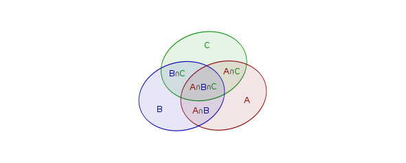
Then the area of the union A ∪ B ∪ C is equal to the sum of the areas A, B, C minus the twice-covered areas A ⋂ B,A ⋂ C,B ⋂ C, but with the addition of the three-times covered area A ⋂ B ⋂ C: S (A ∪ B ∪ C) =S (A) +S (B) +S (C) -S (A⋂B) -S (A⋂C) -S (B⋂C) +S (A⋂B⋂C)
In a similar way, it is generalized to the union of n sets.
2.5.1. A special case of the theorem on inclusions and exceptions
In some cases, the number of objects that have a certain set of properties depends only on the number of these properties. Then the formula for counting the number of objects that do not have any of the selected properties is simplified.
For arbitrary n we have: N (n) =n! -Cn1*N (1) +Cn2*N (2) -…+ (-1) nN (n)
In the general case, when rearranging n objects, the number of arrangements in which no object is located on in its place: N (n) =n! -Cn1* (n-1)! +Cn2* (n-2)! -…+ (-1) n0!=Dn
The resulting value of Dn is sometimes called a complete disorder formula or sub-factor. The subfactorial Dn can also be represented as follows: Dn=n! [1- (1) / (1!) + (1) / (2!) — (1) / (3!) +…+ (-1) n/ (n!)]
where the expression in […] tends to e-1 with an unlimited increase in n.
A subfactorial has properties similar to those of a regular factorial. For example:
— n!= (N-1) [(n-1)!+ (N-2)!] — for a regular factorial;
— Dn= (n-1) [Dn-1+Dn-2] — for the sub-factorial.
Subfactorials are calculated by the formula: Dn=nDn-1+ (-1) n
2.5.2. Caravan
Problem Let us consider a problem in which a solution can be obtained using the main combinatorics theorem.
Task: 9 camels go in a bargain. How many combinations of camel rearrangements exist, in which no camel follows the one he followed earlier?
We distinguish the forbidden pairs: (1, 2), (2, 3), (3, 4), (4, 5), (5, 6), (6, 7),
(7, 8), (8, 9) To solve, we apply the main theorem of combinatorics.
To do this, we define what an object is and what properties are. By objects we mean various arrangements of camels. In total there will be N = 9!. By properties we mean the presence of a certain pair
in the permutation. Thus, the number of properties is 8. Then the number of permutations that do not have any of the 8 properties: N (8) =9! -C81*8!+C82*7! -C83*6!+C84*5! -C85*4!+C86*3! -C87*2!+C88*1!=142729=D9=D8
In the general case, for n camels, we have: Dn+Dn-1
2.5.3. Problem about disturbances
Set we denote all permutations by S, and the list of properties will consist of properties pi: property pi is the property of this or that substitution to leave elementin place i. It is clear that disorder is just such a permutation that does not have any properties from P= {p1,…,pn}. Following the inclusion-exclusion formula, we get: N=M-∑i=1nS(pi)+∑i,jS(pipj)-...+(-1)k∑pi1,pi2,...pik,S(pi1,pi2,...pik)+...+(-1)nS(p1,p2,...pn) =n! -Cn1 (n-1)!+Cn2 (n-2)! -…+ (-1) kCnk (n-k)!+…+ (-1) n=n! (1—1+ (1) / (2!) — (1) / (3!) +…+ (-1) k/ (k!) +…+ (-1) n/ (n!)) ≈ (n!) / (e).
2.6. The concept of a lattice, a distributive lattice
A lattice is a partially ordered set in which each two-element subset has both an exact upper (sup) and an exact lower (inf) face. This implies the existence of these faces for any nonempty finite subsets.
Any two elements in such a partially ordered set must be comparable: ∀a,b must be either a ≤ b ∨ b ≤ a.
Precision (smallest) of the upper edge (boundary) or supremum subset X ordered set (or class) M, is the smallest element M, which is equal to or more than all of the elements of X.In other words, the supremum is the smallest of all the upper faces.
More ∈ formally: SX= {yM | ∈ ≤
the set of upper bounds of X, that is, elements of M, equal to or greater than any element X.
s=sup sup X ⇔ ∈ s Sx ∧ ∀y ∈ Sx: s ≤ y)
H=sup sup (a,b) = ∧ — the exact upper face of the two elements.
Precision (maximum) of the bottom face (boundary) orinfimum subset X of an ordered set (or class) M, is called the largest element M, which is equal to or less than all of the elements of X.In other words, the infimum is the largest of all the lower faces.
L=inf inf (a,b) = ∨ — the exact lower bound of the two elements.
Theorem: if the lower (upper) face exists, then it is unique.
Proof: x=inf inf (a,b) ∧ y =inf inf (a,b) ⇒ y≤x ∧ x≤y ⇒ x=y
THEOREM IS PROVED.
A lattice is called distributive if sup and inf are distributive:
a∪ (b⋂c) = (a∪b) ⋂ (a∪c),a⋂ (b∪c) = (a⋂b) ∪ (a⋂c), (2.6.4)
Lemma: the set of natural numbers N+ is a lattice with respect to operations ≤,max, min.
Proof: by definition, a lattice is a partially ordered set. Let us show that the set of natural numbers is a partially ordered set. Moreover, a linearly ordered set.
Consider the relation ≤. This is a relation of order because it is:
— Reflective:∀a ∈ N,a ≤ a
— Transitive: ∀a,b,c ∈ N,a ≤ b ⋂ b ≤ c ⇒ a ≤ c
— Antisymmetric: ∀a,b ∈ N,a ≤ b ⋂ b ≤ a ⇒ a = b
In addition, there are many natural numbers linearly ordered, because: ∀a,b ∈ N,a ≤ b ⋂ b ≤ a)
To prove that the set N is a lattice, it remains to show that for any two-element subset X ⊂ N there are exact upper and lower faces. This follows from linear ordering. X= {a,b}
Supposeb a ≤ b. Then: in fX=a, supX=b
Similarly, we can reason for another case.
APPROVED PROVEN
2.7. The principle of mathematical induction
Formulation: suppose that it is required to establish the validity of an infinite sequence of statements numbered by natural numbers: P (1),P (2),…,P (n),P (n+1).
Assume that:
— It is established thatP (1) is true (this statement is called the base of induction).
— For anyn, it is proved that ifP (n) is true, thenis trueP (n +1) (this statement is called the induction transition).
Then all the statements of our sequence are true.
Proof:
— induction basis. Let P (1) be true, i.e.holds P (k) for some k ∈ N+.
— inductive step. If (P + k) — true, then ∀n ∈ N+ P (n) — true.
We prove that the method of mathematical induction can be applied using the method of proof by contradiction. Suppose that for some numbers in the natural series the method of mathematical induction is incorrect.
Let them form the set N» ⊆ N+. N+ is a lattice with respect to the operations ≤,max, min (by the lemma proved in Section 2.6); therefore, N», as its subset, is also a lattice ⇒ ∃m | ∀k ∈ N»(m,k) =m.
— If m = 1, then a contradiction with (a) the condition.
— If m ≠ 1, then (m — 1) is not natural.
P (m — 1 +1) is true (by condition (b)); therefore, P (m) is true (a contradiction to condition (b)).
PRINCIPLE PROVED
2.8. The Cantor diagonal method
If each element of the set X corresponds to a single element from the set Y, then it is said that a one-to-one correspondence is established between these sets.
Consider 2 infinite sets: the
— set of natural numbers 1, 2, 3, 4, 5, …, n, …;
— the set of even positive integers 2, 4, 6, …, 2n, … (this is a subset of the first set).
Since a series of even numbers can be numbered using natural numbers, a one-to-one correspondence can be established between these two sets. If a one-to-one correspondence cannot be established between a set and its certain subset, then the set is finite.
A set equivalent to a set of natural numbers is called countable. In other words, a countable set can be established one-to-one correspondence with a set of natural numbers.
Theorem: the set of real numbers of the interval [0, 1] is uncountable.
Proof (by diagonalization method): each number is represented as an infinite decimal fraction: 0. a1 a2 a3… consisting of digits and not having a period of 9. Suppose that some countable set (of all or only some) of real numbersalying on the interval [0, 1]. Then they can be arranged as a list of lines:
0. a11 a12 a13 a14…
0. a21 a22 a23 a24…
0. a31 a32 a33 a34…
…
Consider the sequence of numbers: b1≠a11,b2≠a22,b3≠a33,…,not equal to 9. Then the number 0. b1 b2 b3is… not in the list, although it is in the interval on the segment [0, 1]. This means that all real numbers from this segment cannot be enumerated using natural numbers. Thus, no countable set of real numbers lying on the segment [0, 1] does not exhaust this segment.
THEOREM IS PROVEN.
2.9. The principle of transfinite induction
Transfinite induction is a method of proof that generalizes mathematical induction to the case of an uncountable number of parameter values.
Transfinite induction is based on the following statement.
Statement: let a completely ordered setbe given A. P (x),x ∈ A is a statement. Suppose that for each element of the set A, since P (y) is true for all y <x, it follows that p (x) is true. Then the statement P (x) is true for any x.
Mathematical induction is a special case of transfinite induction. Indeed, let M be the set of natural numbers. Then the statement of transfinite induction turns into the following: if for any positive integer n the truth of statements P (1), P (2), …, P (n — 1) implies the truth of statement P (n), then all statements P (n) Moreover, the induction base, that is, P (1), turns out to be a trivial special case for n = 1.
2.10. Newton’s binomial
2.10.1. Case of two variables
Formula (Newton’s binomial). A formula for decomposing into separate terms a non-negative integer power of the sum of two variables, having the form: (a+b) n=∑k=0nCnkankbk
Proof (by induction). We have the formula: (a+b) n=∑k=0nCnianibi= Cn0an+ Cn1an-1b1+…+Cnna0bn
Induction base: for n = 2, the statement is obvious: (a+b) 2=C20a2b0+ C21a1b1+C22a0b2=a2+2ab+b2
Induction step: suppose that the statement is true for n — 1 and show that it will be true for n. (a+b) n-1=∑i=0n-1Cn-1ian-1-ibi
(a+b) n= (a+b) n-1* (a+b) = ∑i=0n-1Cn-1ian-1-ibi* (a+b)
Which is equivalent: (Cn-10an-1b0+Cn-11an-2b1+…+Cn-1n-1a0bn-1) * (a+b)
And: Cn-10anb0+Cn-11an-1b1+…+Cn-1n-1a1bn-1+Cn-10an-1b1+Cn-11an-2b2+…+Cn-1n-1a0bn
Group the terms: Cn-10an+ (Cn-10+Cn-11) an-1b1+…+Cn-1n-1bn
Using the proven earlier identity Cnk=Cn-1k+ Cn-1k-1 we get:
Cn0an+Cn1an-1b1+Cn2an-2b2+…+Cnnbn
WHAT YOU NEED TO PROVE.
2.10.2. Ordered partitions and the generalized
Newton bin recall that a partition of a set A is the family {Ai} of its pairwise disjoint subsets such that: ∪i Ai=A. Thesubsets Ai are called partition blocks. If the family takes into account the order of the subsets, then it is called an ordered partition. We say that the ordered partition (A1,A2,…,Am of the) set E= {e1,e2,…,en} is of type (k1,k2,…,km) if |A1|=k1,|A2|=k2,…,|Am|=km. The number of such partitions is denoted by P (k1,k2,…,km) or Pn (k1,k2,…,km), where n=k1+k2+…+km.
Pn (k1,k2,…,km) = (n!) / (k1!k2!…km!)
This is the number of permutations with repetitions. For the proof of this formula, see §2.4.
Theorem: (x1+x2+…+xm) n=n!∑k1+k2+…+km=n ((1) / (k1!k2!…km!)) x1k1x2k2…xmkm
Proof: we consider how the boxes are factors of the product: (x1+x2+…+xm) (x1+x2+…+xm) … (x1+x2+…+xm)
The product consists of terms of the form x1k1x2k2…xmkm. Each such term occurs as many times as there are ordered partitions of many boxes. The partition will consist of the following subsets: the first subset consists of boxes from whereselected x1 is, the second consists of subsets from whereselected x2 is, etc. Hence, the coefficient at x1k1x2k2…xmkm will be equal to P (k1, k2, ⋅⋅⋅, km).
Q.E.D.
2.11. The Dirichlet Principle
Formulation of1: «if m rabbits planted in n cell, at least one cell is at least |m/n| rabbits, as well as in at least one cell is no more than |m/n| rabbits.» In this formulation, the concepts of «ceiling» and «floor» are used, introduced by D. Knut.
Proof (by contradiction): suppose there are no containers with less than |m/n| objects, that is, in each of the containers there are more than |m/n| objects, we multiply this number by the number of containers and we obtain that the number of objects is more than m, which is unacceptable.
PRINCIPLE PROVED.
If we want to apply the Dirichlet principle in solving a specific problem, then we have to figure out what are «cells» in it and what are «hares».
Formulation 2: «for any total mapping of the set Pcontaining n +1 elements to the set Qcontaining n elements, there are two elements of the set Phaving the same image.»
Using the Dirichlet principle, the existence of an object is usually proved without indicating, generally speaking, the algorithm for finding or constructing it. This gives the so-called non-constructive proof — we cannot say in which particular cage two hares are sitting, but we only know that such a cage exists.
2.12. FermatSmall Theorem
Formulation: if p is a prime, then for any integer non-negative a the difference ap-a is divisible by p, i.e.: (ap-a) mod p=0.
Proof (by induction):
— p = 1: 0 = 0.
— p = 2: (a2-a) =a (a-1) — obviously divided in half, because this is the product of two consecutive natural numbers.
— p = 3: (a3-a) =a (a2—1) =a (a+1) (a-1) — similarly.
We take an arbitrary p and induction on a: (a+1) p- (a-1) = (a+1) p-a-1=∑k=0pCpkak-a-1=∑k=1pCpkak-a
Since both terms:∑k=0p-1Cpnak+ (ap-a)
are divided by p, that is: (∑k=1p-1Cpkak) / (p) + (ap-a) / (p)
then the result will also be divided by p.
THEOREM IS PROVEN
Corollary 1: without any restrictions on a ∈ Z: ap≡a (mod p)
Proof: we multiply both sides of the comparison ap-1≡1 (mod p) by a. It is clear that we get a comparison that holds for amultiple of p.
THE CONSEQUENCE IS PROVED.
Corollary 2: (a+b) p ≡ap+bp (mod p)
2.13. Chinese remainder theorem
Formulation: if the natural numbers a1,a2,…,an are pairwise coprime, then ∀r1,r2,…,rn | d ≤ ri ≤ ai there is a number N, which when divided by ai gives the remainder ri.
Proof (by induction): induction on N.
For N = 1, the statement is obvious: N= aia+ri. Let the statement be true for k,d= a1,a2,…,ak-1. Consider the numbers N, N + d, N +2d, …, N + (ak — 1) d. Let us prove that at least 1 of these numbers gives the remainder rk when divided by ak.
Let’s go from the opposite. Let it not be so. Since the number of numbers in this record is equal to ak, and the possible residues when divided by ak are (ak — 1) pieces. Thus, it follows that of these two numbers according to the Dirichlet principle there are 2 numbers having the same residues. Denote these numbers by (N + sd) and (N + td),0≤s,t≤ak-1. Consider the difference of these numbers: (N+sd) — (N+td) =d (st)
This number is divided by ak. But this is impossible, because: 0≤s,t≤ak, d= a1,a2,…,ak-1. Since the numbers d= a1,a2,…,ak are coprime, the difference (s — t) and d are also coprime with ak. We get a contradiction.
THEOREM IS PROVEN.
2.14. Prufer Code
Let there be a tree (i.e. a connected graph without cycles) with N vertices, numbered from 1 to N (N ≥ 2). The Prüfer code for this tree is constructed as follows: from all hanging vertices (i.e., from vertices adjacent to exactly one edge), the vertex with the lowest number is selected. Then this vertex and its adjacent edge are removed from the graph, and the number of the vertex with which it was adjacent is recorded. In the resulting graph, the hanging vertex with the lowest number is again selected, deleted, and so repeated until only one vertex remains. It is obvious that the result will be a unique vertex number N.The described set of numbers (N — 1 number, each ranging from 1 to N) is called the Prufer code of this graph.
Lemma: for any sequence of length n — 2 from numbers from 1 to n, we can construct a labeled tree for which this sequence is the Prüfer code.
Proof (by induction): base: n = 1 — true. The transition from n to n +1. Let there be a sequence: A= [a1,a2,…,an-2].
We choose a minimum number of v does not lie in A. By the previous lemma, v is the vertex that we deleted first. Connect v and a with1 edge. Remove from the sequence A the number a1. We renumber the vertices, for all ai> v we replace ai with ai-1. And now we can apply the induction hypothesis.
The lemma is proved.
Unpacking the Prufer code is performed by the following function.
Unpacking function (T — code):
— V consists of vertices {v1,v2,…,vn} such that the number of the vertex vi is i, where n is the length of the code T plus 2;
— B= [1,n+2];
— for i from 1 to n +1 — a cycle:
— b= {k ∈ B,k ≠ aj ∀ j ≥ i};
— T=T ∪ {b, ai};
— B=B/ {b};
— Returns T.
2.15. Fibonacci
Numbers Fibonacci numbers — elements of a numerical sequence: 0, 1, 1, 2, 3, 5, 8, 13, 21, 34, 55, 89, 144, 233, 377, 610, 987, 1597, 2584, … — in which each subsequent number is equal to the sum of the two previous numbers. The sequence of Fibonacci numbers is given by a linear recurrence relation: F0=0,F1=1,Fn=Fn-1+Fn-2
(Fn+1) / (Fn) = φ
where φ = (1+√5) / (2) is the «golden ratio».
Sometimes Fibonacci numbers are also considered for negative numbers n as a two-sided infinite sequence: Fn=Fn+2-Fn+1
It is easy to show that: F-n= (-1) n+1Fn
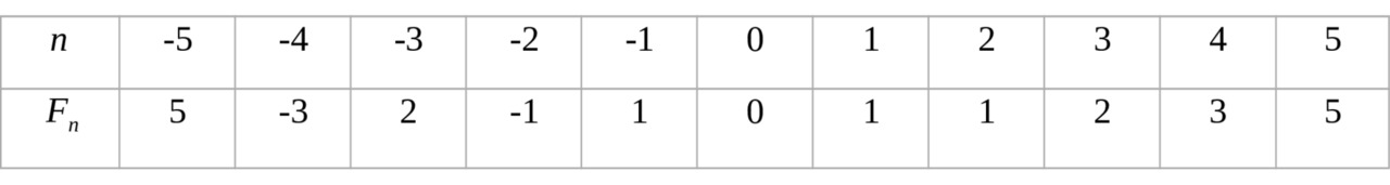
2.16. Bene formula
The bene formula explicitly expresses the value of Fn as a function of n: Fn= (((1+√5) / (2)) n- ((1-√5) / (2)) n) / (√5) = (φn- (-φ) -n) / (φ- (-φ) -1) = (φn- (-φ) -n) / (2φ-1)) Fn
where φ = (1+√5) / (2) is the «golden ratio».
Moreover, φ and (-φ) -1 =1-φ are the roots of the characteristic equation x2-x-1=0.
From the Bene formula it follows that for all n ≥ 0, Fn is theclosest to (φn) / (√5) integer, that is, Fn = [(φn) / (√5)]. In particular, as n → ∞, the asymptoticsholds Fn ~ (φn) / (√5).
The Bene formula can be analytically continued as follows: Fz = ((1) / (√5)) (φz- ((coscosπz) / (√5)))
Moreover, the relation Fz+2=Fz+1+Fz holds for any complex number z.
2.17. Euclidean Lemma
Formulation: if (xy) modp=0, then either x mod p=0, or y mod p=0.
Alternative wording: if a prime p divides without a remainder the product of two integers x*y, then p divides without a remainder either x or y.
Proof (by contradiction): let (xy) mod p=0, but x mod p ≠ 0 (x*y is divisible by p, but x is not divisible by p). Then x and p are coprime, therefore, there are integers u and vsuch that (by the Bezout relation): x*u+p*v=1
Multiplying both sides by y, we obtain: (x*y) *u+p*v*y=y
Both terms of the left side are divided by p, which means that the right side is divided by p. It is proved similarly for the other case (x is divisible byremainder p by).
The lemma is proved.
Corollary (the main theorem of arithmetic): every natural number> 1 can be represented in the form n=a1a2...an, where a1a2...an are prime numbers, and such a representation is unique up to the order of the factors: n> 1:n=p1a1*p2a2*pnan, ∀pi is prime, ai is positive integer.
Proof: let’s go from the opposite. Let n be the smallest positive integer indecomposable into a product of primes, not 1. It cannot also be a prime. If n is a composite number, then it is the product of two smaller positive integers. Since n is the smallest positive integer that cannot be decomposed into a product of primes, it follows that the factors into whichdecomposable are n is, in turn, decomposable. And, therefore, n is also a product of primes. Got a contradiction.
THE CONSEQUENCE IS PROVED
2.18. Stirling numbers
The number of partitions of an m-element set into n blocks is called the Stirling number of the second kind and is denoted by S (m, n). By definition, we put: S (m,0) =0,m> 0
S (m,m) =1
S (0,0) =1
S (m,n) =0,n> m
For other values of the arguments S (m,n) =S (m-1,n-1) + nS (m-1,n)
The number of surjective functions, that is, the number of placements of m items in n boxes, such that all boxes are occupied, is called the Stirling number of the first kind and is denoted s (m, n).
We give definitions of the core of a relation and function.
If R ⊂ A × B — the ratio of A to B, then R*R-1 is called the kernel relationship R.Kernelratio R of A to B is the ratio at A. Every function, being an attitude, has a kernel. The kernel of f is denoted by ker ker f:f*f-1.
Each partition of the set {1,2,…,m} corresponds to the kernel of the surjective function and vice versa. Thus, the number of different kernels of surjective functions is the Stirling number of the second kind, that is, the number of partitions {1,2,…,m}. According to the basic rule of combinatorics: S (m,n) =n!S (m,n) — the number of surjective functions with a given kernel is equal to the number of permutations of the set of values of the function.
Theorem: the following property of Stirling numbers of the second kind holds: S (n,k) =S (n-1,k-1) + kS (n-1,k),0 <k <n
Proof: we prove the last relation. The set of partitions of the set {1,2,…,n} consists of two classes:
— partitions containing the block {n};
— partitions for which n belongs to blocks having more than one element.
In the first class, S (n — 1, k — 1) partitions. In the second class, we get kS (n-1, k) partitions, for each partition of the set {1,2,…,n-1} into k blocks B1,B2,…,Bk corresponds to k partitions.
B1 ∪ {n}, B2, ⋅⋅⋅, Bk,
B1, B2 ∪ {n}, ⋅⋅⋅, Bk,
…
B1, B2, ⋅⋅⋅, Bk ∪ {n},
Therefore, S (n,k) =S (n-1,k-1) + kS (n-1,k) for 0 <k <n
RATIO PROVEN.
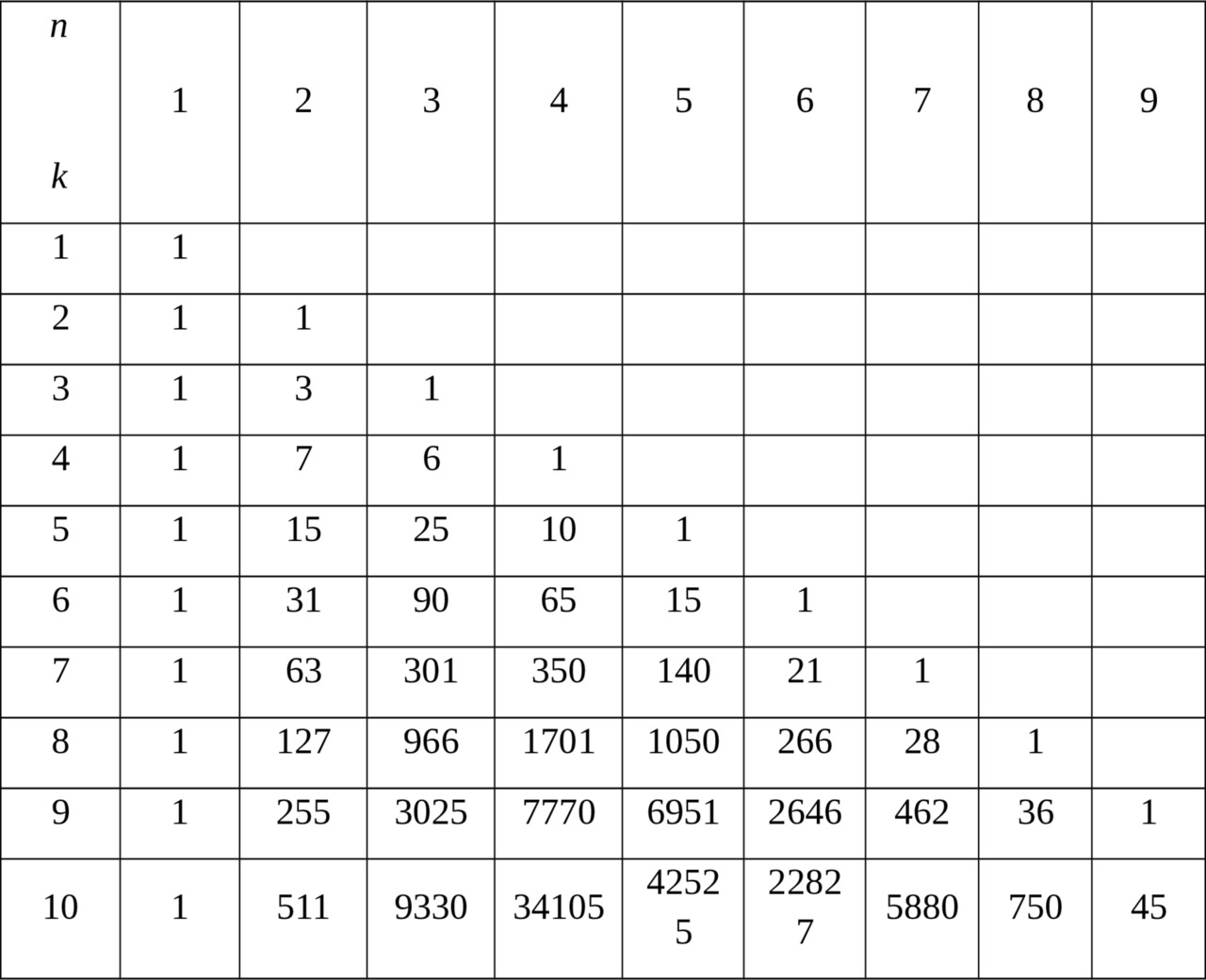
Example: find the number of surjections {1, 2, 3, 4, 5, 6} → {1, 2, 3, 4}. It is equal to 4!S (6,4). The number S (6,4) is found from the table. Hence the desired number is 4!*65=1*2*3*4*65=1560.
2.19. Bell Number
The number of all partitions of an m-element set is called the Bell number and is denoted by B (m).
B (m):= ∑n=0m S (m,n),B (0):=1
2.20. Generating functions
Let {ak} be a sequence of numbers, where k ≥ 0 run through non-negative integer values. The generating function a (x) of the sequence {ak} is the sum of a series: ∑k=0∞akxk
Sometimes the sum is taken over all positive integers k ≥ 1. This occurs when the number a0 undefined.
For example, (1+x) n= ∑k=0nCnkxk
The generating functions are used in the proof by the method of uncertain coefficients, the essence of the method is that the form of the factors into which the given polynomial is decomposed is guessed, and the coefficients of these factors (also) are determined by multiplying the factors and equating the coefficients for the same degrees of the variable.
The theoretical basis of the method is the following statements:
— two polynomials are equal if and only if their coefficients are equal;
— any polynomial of the third degree has at least one real root, and therefore it decomposes into a product of a linear and quadratic factor;
— any polynomial of the fourth degree is decomposed into a product of polynomials of the second degree. ((A (x) = ∑aiφi (x)) / (B (x) = ∑biφi (x))) and A=B ⇒ ∀i ai=bi
2.20.1. Properties of generating functionsterminated
Power series can be integrallyand differentiated inside the circle of convergence. In particular, differentiating and integrating Newton’s bin, we obtain: ∑k=1∞kCnkxk-1=n (1+x) n-1
∑k=0∞Cnk ((xk+1) / (k+1)) = (((1+x) n+1—1) / (n +1))
Example: recall formula for the sum of an infinite geometric series:
∑k=0∞a0qk=a0limn→∞∑k=0nqk=a0limn→∞ (1-qn+1) / (1-q) =a0 (1) / (1-q)
We find the generating function for the sequence when a0 = 1: ∑k=0∞xk= (1) / (1-x)
Termwise differentiation equation:1++xx2++…xn+…= (1) / (1-x)
Leads to generating functions for the sequence an = n +1: 1+2x+3x2+…+ (n+1) xn+…= (1) / (1-x) 2
Integration by term leads to the generating function of the sequence (1) / (n): x+ ((x2) / (2)) +…+ ((xn) / (n)) = ∫0x (dx) / (1-x) =ln (1-x)
The following properties of generating functions take place.
With each sequence a0,a1,…,an,… you can associate a series: A (t) = a0+a1t+…+antn+…
called the generating function for the sequence {an}.
In those cases when the series A (t) converges to some function f (t), the function f (t) is also called the generating for {an}. In problems of finding the generating function for the sequence {an}, it is usually meant to find the function f (t), whose Maclaurin series is A (t). The exponential generating function for {an} is the series: E (t) = a0+a1 (t) +…+ ((ant) / (n!)) +…
It is possible to define the operations of addition, multiplication by a constant for generating functions, considering them as formal series.
Let A (t) and B (t) — generating functions for sequences {an} and {bn},respectively, α and, β — are constants. Then: αA (t) + βB (t) = αa0 + βb0 + (αa1 + βb1) t +…+ (αan + βbn) tn +…,
A (t) * B (t) = a0b0 + (a0b1 + a1b0) t +…+ (a0bn + a1bn-1 + anb0) tn +…
2.20.2. Partitions of numbers
A partition of a natural number n into k terms is an equivalence class of sequences of positive integers (b1,b2,…,bk) such that: n= b1,b2,…,bk, k> 0, b1,b2,…,bk> 0
Two sequences are considered equivalent if they differ by a permutation of the elements bi. Each equivalence class can be represented uniquely as a non-increasing sequence a1≥a2≥…≥ak such that a1+a2+…+ak=n. Let P (n, k) be the number of partitions of n into k terms.
Then the number of all partitions is: P (n):=∑k=1nP (n,k),n> 0
We assume by definition: P (0) =P (0,0) =1.
Example:
— P (5) = 7:
— 5 = 5;
— 5 = 4 +1;
— 5 = 3 +2;
— 5 = 3 +1 +1;
— 5 = 2 +2 +1;
— 5 = 2 +1 +1 +1;
— 5 = 1 +1 +1 +1 +1.
The Ferres diagram for a1+a2+…+ak=n consists of k lines in the i-line containing ai points. For example, for 5 = 2 +2 +1, the Ferres diagram shown in Figure 2.3.
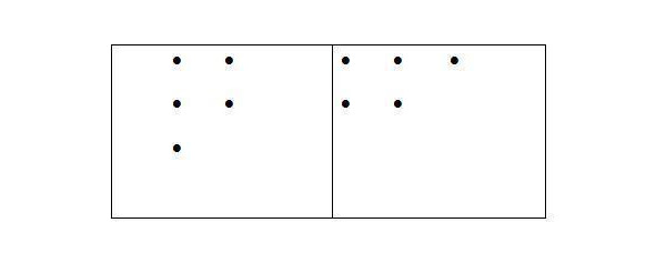
In this figure, the second Ferres diagram is conjugated to the first.
Lemma: the number of partitions P (n) is equal to the number of solutions (λ1,λ2,…,λn) of the equation λ1*1+λ2*2+…+λn*n.
Proof: if among the numbers a1≥a2≥…≥ak, the partition of n contains и1 — units, L2 — twos, …, Ln — n-ok, then we get the solution to the equation. It is clear that this correspondence is one-to-one.
The lemma is proved.
Denote by Ph (n) the number of partitions of n into terms not greater than h.
Theorem: the generating function of the sequence of partition numbersPh (0),Ph (1),Ph (2),… is: ∏k=1h (1-xk) -1
Proof: the product is: (1+x+x2+…) (1+x2+x4+…) (1+x3+x6+…) … (1+xh+x2h+…)
If we multiply the contents of the brackets, we get a polynomial equal to the sum: xλ1*x2λ2*…*xhλn
Hence the coefficient at xn is equal to the number of sequences (λ1,λ2,…,λn) for which: λ1*1+λ2*2+…+λn*h=n.
It will be equal to the number of partitions of n into terms not greater than h.
THEOREM IS PROVEN
Corollary: the generating function of the sequence of partition numbers P (0),P (1),P (2),… is: ∏h=1∞ (1-xh) -1
2.20.3. Catalan numbers
A root tree, each vertex of which has at most two children, is called binary, if the children are assigned an additional attribute of a «left» or «right» adjacent vertex. A vertex cannot have two left or two right adjacent vertices. A binary tree, together with a function that maps each vertex to a certain number, is called a binary tree of numbers.
The binary tree of numbers can be determined by induction. An empty tree is a binary tree of numbers. If T1 and T2 are binary number trees, then (T1, number, T2) is a binary tree of numbers.
Define the equivalence relation on a set of binary trees numbers S ~ T as follows:
— If S=T=∅,then S ~T.
— If S= (S1,m,S2),T= (T1,n,T2),S1 ~T1 andS2 ~T2 then S ~T
The number of equivalence classes of binary trees with n vertices is called n- m is the Catalan number and is denoted by cn.
The equivalence classes of binary trees having n vertices, where n = 0, 1, 2, 3 are shown in Figure 2.4.
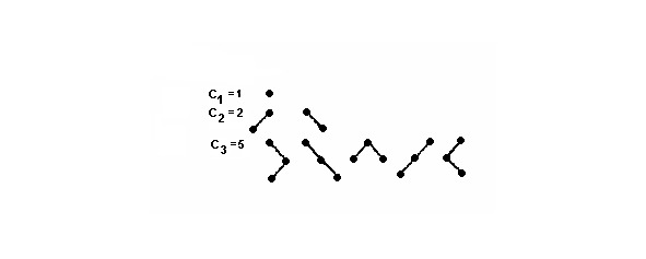
Example: a family tree, where father and mother are indicated for each element, is a binary tree if the property of being a father for v is attributed to the left adjacent vertex, and to be the mother is right.
Example: the number of parentheses. Let * be a binary operation on the set A, which is not assumed to be commutative or associative. The term is determined by induction. In normal Backus-Naur form, the definition will be as follows: TERM:: = a | (TERM * TERM), where a ∈ A is an arbitrary element.
For example, the terms are the words: (a * a) * b, a * (b * c), etc. The number of terms containing n operations * is equal to cn.
The binary trees shown in Figure 2.20.1 correspond to the terms:
— a;
— (a * b);
— ((a * b) * c), (a * (b * c));
— (a * ((b * c) * d)), (a * (b * (c * d))), ((a * b) * (c * d)), (((a * b) * c) * d), ((a * (b * c)) * d).
Example: elements of an increasing sequence of n numbers can be located in the nodes of the search tree. It will be a binary tree and can be selected inn ways.
Theorem: Catalan numbers are equal: Cn= ((1) / (n+1)) C2nn
Proof: there are relations for class numbers of binary trees: Ck=C0Ck-1+C1Ck-2+…+Ck-1 C0,k> 0
Let C (x) =∑k=0∞ckxk be the generating function of a sequence of Catalan numbers. We obtain: C (xx) =C2 (x) +1
() ((√) / ()) Where: Cx=1-1-4x2x= ∑1∞ ((1) / (k)) C2k-2k-1xk-1= ∑k0∞ ((1) / (k+1)) C2kkxk
THEOREM IS PROVED.
Problem (walk on the half-line): a classical problem in which Catalan numbers are encountered. Let’s consider a straight line. Some object is on a straight line at position 0. It can move in one step either to the left or to the right by one position. In how many ways can one move from the initial position to it in2nsteps so that it never turns out to be left of zero?
First, we consider the case when the zero mark can be crossed (the problem of wandering on a straight line). In this case, you need to perform2nsteps, nof which are done to the left andn — to the right (in any sequence). Denote by the symbol 0 the movement to the left, and by the symbol 1 the movement to the right. How many sequences of zeros and ones exist in which zeros and ones are exactly inn? This is the number of combinations: ((2n) / (n))
Now we consider the case when movement to the left of zero is forbidden. In this case, at each step it is required that the number of steps already taken to the left be no more than the number of steps already taken to the right. Imagine that a step to the right is an opening bracket, and a step to the left is a closing bracket. Then any path from 0 to 0 that does not cross the left border can be represented by a regular bracket sequence. Conversely, any correct sequence will set the path. Thus, the number of walks on the half-line is the quantity Cn= ((1) / (n+1)) ((2n) / (n))
2.21. Generalized recurrence relations
Let us consider the generalization of Fibonacci sequences. The formula: un+r=C1un+r-1+C2un+r-2+…+Crun, (2.21.1)
is called a homogeneous linear recurrence equation of order r.
Its solution is the sequence {un}, uniquely determined by the initial values u0,u1,u2,…,ur-1. The solution to this equation is called a return or recurrence sequence of order r.
Example: geometric progression is a solution to the equation: un+1=qun
Its members are described by the formula: un=u0qn
Hence the geometric progression is a return sequence of order 1.
Example: Arithmetic progression: un=u0+nd satisfies relation: un+1-un=un+2-un+1
We obtain a homogeneous recurrence equation: un+2=2un+1-un
The initial data are given by the values u0 and u1=u0+d. Hence, the arithmetic progression is a return sequence of order 2.
We find the generating function: u (x) =∑k=0∞ukxkof the return sequence (2.21.1). We denote: K (x) =1-c1x-c2x2-… -crxr
Example: an arbitrary periodic sequence is a return sequence of order psatisfying the recurrence relation: un+p=un, where p is the period of the sequence.
Theorem: the product u (x) *K (x) =D (x) is a polynomial of degree less than r.
Proof: we calculate the coefficient of the series D (x) for xn + r. For n ≥ 0 it will be equal to: un+r- (C1un+r-1+C2un+r-2+…+Crun) =0
Hence D (x) is a polynomial of degree less than n.
THEOREM IS PROVEN
Note: the quotient of the division of any two polynomials is a generating function of some return sequence whose order is equal to the degree of the denominator.
In the general case, the numbers〈i in the expansion: K (x) = (1-a1x) (1-a2x) … (1-arx)
are the roots of the equation: F (a) =ar-c1ar-1-… -cr-1a-cr=0
because: K (x) =xrF ((1) / (x))
If all the roots of the equation F (a) =0 are real and different, then we get: (D (x) /K (x)) = ((A1) / (1-a1x)) + ((A2) / (1-a2x)) +…+ ((Ar) / (1-arx))
From: un=A1a1n+…+Arrarn
This allows us to compose a system of linear equations for finding Ai using the known values u0,u1,…,ur-1. If there are multiple roots, then using the formulas for the derivatives of geometric progression, we can prove that the solution will be supplemented by the terms: A1ain+ nA2ain+…+nk-1Akain, where k is the multiplicity root 〈i.
2.22. Zhegalkin polynomial
Zhegalkin polynomial is the sum modulo two (exclusive OR operation) products (conjunctions) of non-inverted variables, as well as (if necessary) constants 1. We consider formulas over the class K= {x1x2,x1 ⊕ x2,0,1}.
The Zhegalkin polynomial (reduced polynomial) is the representation of the binary function f (x1,…,xn) by the formula of the form: f (x1,…,xn) =a0 ⊕ ∑i=1nai*xi ⊕ ∑ {i,f} 1 ≤ i ≤ j ≤ naij*xi*xj ⊕…⊕ a1…n*x1*…*xn
where: a0,a1,…,an, a12,…,a1…n ∈ F2
There aretotal 2 innterms. Recall that + now means addition modulo 2, the coefficientsa0,a1, … are constants (equal to zero or one).
Example: let the function: f (x1,x2,x3) =x1x3 ∨ x2x3
while: f (x1,x2,x3) =x1*x3 ⊕ x2*x3 ⊕ x1*x3*x2*x3=x1*x3 ⊕ x2*x3= (x1 ⊕ 1) *x3 ⊕ x2* (x3⊕ 1) that is: x2⊕x3⊕x1*x3⊕x2*x3
Theorem: Any function n ofvariables can be represented by a polynomial Zhegalkin and this representation is unique.
Proof: any function f (x1,x2,…,xn) has its own truth table. First, we write this function in the form of the Zhegalkin polynomial with indefinite coefficients. Then, in turn, we substitute various sets of variables and find the coefficients. It is easy to see that for each substitution we find only one coefficient. Since the number of collections is equal to the number of coefficients (and equal to 2n), this implies the statement of the theorem.
THEOREM IS PROVEN
2.22.1. Construction of the Zhegalkin polynomial from the SDNF
SDNF has the property that for any values of the input variables, at most one expression term is converted to unity. For such expressions, aoperation is disjunctione quivalent to anoperation exclusive OR.
When converting PDNF a polynomial Zhegalkin enoughreplace all disjunctions too peration exclusive-OR and get rid of inversions using equivalent transformation ¬A=A+1, where the summation is performed modulo 2. The following is a scheme for constructing Zhegalkin polynomial for complete disjunctive normal form
— get rid of disjunction rule: x ∨ y = xy + x + y;
— get rid of negatives by the rule: x = x +1;
— open the brackets according to the rule: x (y + z) = xy + xz;
— we present «similar ones» by the rule: x + x = 0.
Recall that summation is carried out modulo 2 everywhere.
2.23. The problem of Hanoi towers
Let us consider the solution of the problem, which is called the problem of Hanoi towers. There is an ancient Indian legend according to which, in the city of Benares, under the dome of the main temple, in the place where the center of the Earth is located, there are three diamond rods on the bronze platform. On the day of creation, 64 rings were put on one of these rods. God instructed the priests to transfer the rings from one rod to another, using the third as an auxiliary. Priests are required to comply with the conditions:
— carry only one ring at a time;
— the ring can be transferred from one rod (x) to another (y) only if it has a smaller diameter than the upper ring located on the rod y, or the rod y is free.
According to legend, when, observing all conditions, the priests will bear all 64 rings, the end of the world will come.
We give an additional, more obvious, formulation of the problem.
Three rods are given ((n) — initial, (k) — final, (e) — additional) on the rod (na number of disks are strung) (we will assume it is equal to n), while all disks have different diameters and are located on the rod (m) in the order of decreasing the diameter from bottom to top as shown in Figure 2.5.
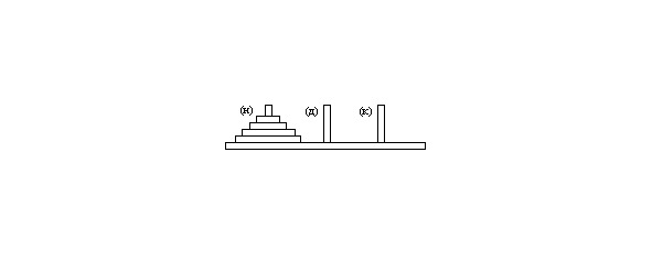
It is necessary to move all the disks to the rod (k), i.e. the puzzle should be brought to the form as in figure 2.6.
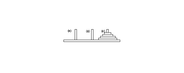
in this case, only one disk can be moved in one move, and as a result of the move there should not be a situation when a disk with a large diameter will be placed on a disk with a smaller diameter as in Figure 2.7.
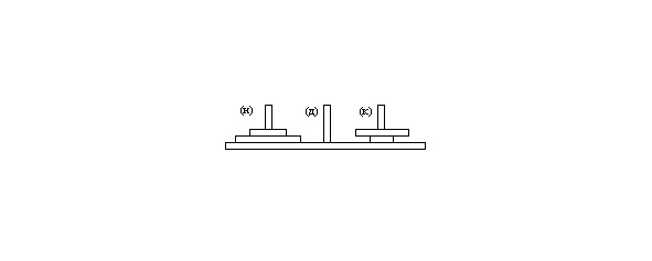
problem The task is to determine the sequence of transfers of rings of minimum length. Solution of the problem will be considered valid hyphenation sequence, each of which has the form: x → y
where x and y one of the symbols B,A, C. If only one ring, the object is achieved for one transfer A → B. To move the two rings is required to perform three → → actions: AC, AB, C →
The solution to the problem for three rings contains seven actions, for four — 15. It is easy to show that for n rings of actions there will be 2n-1.
2.24. The general problem of sticker stamps
There are stamps with denominations of n1,n2,…,nk. How many ways can I pay with their help an amount of N rubles, if two methods that differ in order are considered different? All numbers n1,n2,…,nk are different, and the stock of marks is unlimited. Here, in the first place, we will indicate the number of terms, in the second — the number to be broken, and in the last — restrictions on the value of the terms.
In this case, the number f (N) of the methods satisfies the relation: f (N) =f (N-n1) +f (N-n2) +…+f (N-nk), (2.24.1)
Moreover, f (N) =0 if f (0) =1 and N <0. Using relation (2.24.1), we can find f (N) for any Nby sequentially calculating: f (1),f (2),…,f (N-1).
We consider a particular case of this problem when n1=1,n2=2,…,nk=k. We get all kinds of partitions of N into terms 1,2,…,k, and partitions that differ in the order of terms are considered different. Denote the number of these partitions by φ (k;N). In the first place we will indicate the number of terms, in the second — the number to be broken, and in the last — restrictions on the size of the terms. From relation (2.24.1) it follows that: φ (k;N-1) +φ (k;N-2) +…+φ (k; Nk)
Moreover, φ (k;0) =1 and φ (k;N) =0 if N <0. Calculation φ (N;k) can be simplified if we notice that: φ (N-1;k) =φ (N-2;k) +φ (Nk-1;k)
and therefore: φ (N;k) =2φ (N-1;k) -φ (Nk-1;k)
it is clear that the terms may not be more than N.Therefore, φ (N,N) is equal to the number of all partitions into N into natural terms (including the «partition» N = N). If the number of terms is s, then we obtain CN-1s-1 partitions. Therefore: φ (N,N) = CN-10+ CN-11+…+ CN-1N-1=2N-1
So, we have proved that the positive integer N can be divided into terms 2N-1 in ways. Recall that in this case the order of the terms is taken into account.
2.25. Return search method
Return search is a search method of all possible solutions to find the so-called set of complete solutions. Each partial solution defines a subset of the complete solutions. The return search method is based on the fact that when searching for a partial solution, an attempt is made repeatedly to expand the so-called current partial solution.
The definition of an exhaustive routine should be understood as follows: for all first moves, all kinds of second moves will be sorted, then for second moves all kinds of third moves will be sorted, and so on, until all variants of moves are sorted. Thus, the first suitable option is searched, then the second one for this variant of the move, and so on, until all options are enumerated for the next move.
Бесплатный фрагмент закончился.
Купите книгу, чтобы продолжить чтение.